Super PerformanceThe "Super Performance" script is a custom indicator written in Pine Script (version 6) for use on the TradingView platform. Its main purpose is to visually compare the performance of a selected stock or index against a benchmark index (default: NIFTYMIDSML400) over various timeframes, and to display sector-wise performance rankings in a clear, tabular format.
Key Features:
Customizable Display:
Users can toggle between dark and light color themes, enable or disable extended data columns, and choose between a compact "Mini Mode" or a full-featured table view. Table positions and sizes are also configurable for both stock and sector tables.
Performance Calculation:
The script calculates percentage price changes for the selected stock and the benchmark index over multiple periods: 1, 5, 10, 20, 50, and 200 days. It then checks if the stock is outperforming the index for each period.
Conviction Score:
For each period where the stock outperforms the index, a "conviction score" is incremented. This score is mapped to qualitative labels such as "Super solid," "Solid," "Good," etc., and is color-coded for quick visual interpretation.
Sector Performance Table:
The script tracks 19 sector indices (e.g., REALTY, IT, PHARMA, AUTO, ENERGY) and calculates their performance over 1, 5, 10, 20, and 60-day periods. It then ranks the top 5 performing sectors for each timeframe and displays them in a sector performance table.
Visual Output:
Two tables are constructed:
Stock Performance Table: Shows the stock's returns, index returns, outperformance markers (✔/✖), and the difference for each period, along with the overall conviction score.
Sector Performance Table: Ranks and displays the top 5 sectors for each timeframe, with color-coded performance values for easy comparison.
In den Scripts nach " TABLE " suchen

Seasonality DOW CombinedOverall Purpose
This script analyzes historical daily returns based on two specific criteria:
Month of the year (January through December)
Day of the week (Sunday through Saturday)
It summarizes and visually displays the average historical performance of the selected asset by these criteria over multiple years.
Step-by-Step Breakdown
1. Initial Settings:
Defines minimum year (i_year_start) from which data analysis will start.
Ensures the user is using a daily timeframe, otherwise prompts an error.
Sets basic display preferences like text size and color schemes.
2. Data Collection and Variables:
Initializes matrices to store and aggregate returns data:
month_data_ and month_agg_: store monthly performance.
dow_data_ and dow_agg_: store day-of-week performance.
COUNT tracks total number of occurrences, and COUNT_POSITIVE tracks positive-return occurrences.
3. Return Calculation:
Calculates daily percentage change (chg_pct_) in price:
chg_pct_ = close / close - 1
Ensures it captures this data only for the specified years (year >= i_year_start).
4. Monthly Performance Calculation:
Each daily return is grouped by month:
matrix.set updates total returns per month.
The script tracks:
Monthly cumulative returns
Number of occurrences (how many days recorded per month)
Positive occurrences (days with positive returns)
5. Day-of-Week Performance Calculation:
Similarly, daily returns are also grouped by day-of-the-week (Sunday to Saturday):
Daily return values are summed per weekday.
The script tracks:
Cumulative returns per weekday
Number of occurrences per weekday
Positive occurrences per weekday
6. Visual Display (Tables):
The script creates two visual tables:
Left Table: Monthly Performance.
Right Table: Day-of-the-Week Performance.
For each table, it shows:
Yearly data for each month/day.
Summaries at the bottom:
SUM row: Shows total accumulated returns over all selected years for each month/day.
+ive row: Shows percentage (%) of times the month/day had positive returns, along with a tooltip displaying positive occurrences vs total occurrences.
Cells are color-coded:
Green for positive returns.
Red for negative returns.
Gray for neutral/no change.
7. Interpreting the Tables:
Monthly Table (left side):
Helps identify seasonal patterns (e.g., historically bullish/bearish months).
Day-of-Week Table (right side):
Helps detect recurring weekday patterns (e.g., historically bullish Mondays or bearish Fridays).
Practical Use:
Traders use this to:
Identify patterns based on historical data.
Inform trading strategies, e.g., avoiding historically bearish days/months or leveraging historically bullish periods.
Example Interpretation:
If the table shows consistently green (positive) for March and April, historically the asset tends to perform well during spring. Similarly, if the "Friday" column is often red, historically Fridays are bearish for this asset.

Kripto Fema ind/ This Pine Script™ code is subject to the terms of the Mozilla Public License 2.0 at mozilla.org
// © Femayakup
//@version=5
indicator(title = "Kripto Fema ind", shorttitle="Kripto Fema ind", overlay=true, format=format.price, precision=2,max_lines_count = 500, max_labels_count = 500, max_bars_back=500)
showEma200 = input(true, title="EMA 200")
showPmax = input(true, title="Pmax")
showLinreg = input(true, title="Linreg")
showMavilim = input(true, title="Mavilim")
showNadaray = input(true, title="Nadaraya Watson")
ma(source, length, type) =>
switch type
"SMA" => ta.sma(source, length)
"EMA" => ta.ema(source, length)
"SMMA (RMA)" => ta.rma(source, length)
"WMA" => ta.wma(source, length)
"VWMA" => ta.vwma(source, length)
//Ema200
timeFrame = input.timeframe(defval = '240',title= 'EMA200 TimeFrame',group = 'EMA200 Settings')
len200 = input.int(200, minval=1, title="Length",group = 'EMA200 Settings')
src200 = input(close, title="Source",group = 'EMA200 Settings')
offset200 = input.int(title="Offset", defval=0, minval=-500, maxval=500,group = 'EMA200 Settings')
out200 = ta.ema(src200, len200)
higherTimeFrame = request.security(syminfo.tickerid,timeFrame,out200 ,barmerge.gaps_on,barmerge.lookahead_on)
ema200Plot = showEma200 ? higherTimeFrame : na
plot(ema200Plot, title="EMA200", offset=offset200)
//Linreq
group1 = "Linreg Settings"
lengthInput = input.int(100, title="Length", minval = 1, maxval = 5000,group = group1)
sourceInput = input.source(close, title="Source")
useUpperDevInput = input.bool(true, title="Upper Deviation", inline = "Upper Deviation", group = group1)
upperMultInput = input.float(2.0, title="", inline = "Upper Deviation", group = group1)
useLowerDevInput = input.bool(true, title="Lower Deviation", inline = "Lower Deviation", group = group1)
lowerMultInput = input.float(2.0, title="", inline = "Lower Deviation", group = group1)
group2 = "Linreg Display Settings"
showPearsonInput = input.bool(true, "Show Pearson's R", group = group2)
extendLeftInput = input.bool(false, "Extend Lines Left", group = group2)
extendRightInput = input.bool(true, "Extend Lines Right", group = group2)
extendStyle = switch
extendLeftInput and extendRightInput => extend.both
extendLeftInput => extend.left
extendRightInput => extend.right
=> extend.none
group3 = "Linreg Color Settings"
colorUpper = input.color(color.new(color.blue, 85), "Linreg Renk", inline = group3, group = group3)
colorLower = input.color(color.new(color.red, 85), "", inline = group3, group = group3)
calcSlope(source, length) =>
max_bars_back(source, 5000)
if not barstate.islast or length <= 1
else
sumX = 0.0
sumY = 0.0
sumXSqr = 0.0
sumXY = 0.0
for i = 0 to length - 1 by 1
val = source
per = i + 1.0
sumX += per
sumY += val
sumXSqr += per * per
sumXY += val * per
slope = (length * sumXY - sumX * sumY) / (length * sumXSqr - sumX * sumX)
average = sumY / length
intercept = average - slope * sumX / length + slope
= calcSlope(sourceInput, lengthInput)
startPrice = i + s * (lengthInput - 1)
endPrice = i
var line baseLine = na
if na(baseLine) and not na(startPrice) and showLinreg
baseLine := line.new(bar_index - lengthInput + 1, startPrice, bar_index, endPrice, width=1, extend=extendStyle, color=color.new(colorLower, 0))
else
line.set_xy1(baseLine, bar_index - lengthInput + 1, startPrice)
line.set_xy2(baseLine, bar_index, endPrice)
na
calcDev(source, length, slope, average, intercept) =>
upDev = 0.0
dnDev = 0.0
stdDevAcc = 0.0
dsxx = 0.0
dsyy = 0.0
dsxy = 0.0
periods = length - 1
daY = intercept + slope * periods / 2
val = intercept
for j = 0 to periods by 1
price = high - val
if price > upDev
upDev := price
price := val - low
if price > dnDev
dnDev := price
price := source
dxt = price - average
dyt = val - daY
price -= val
stdDevAcc += price * price
dsxx += dxt * dxt
dsyy += dyt * dyt
dsxy += dxt * dyt
val += slope
stdDev = math.sqrt(stdDevAcc / (periods == 0 ? 1 : periods))
pearsonR = dsxx == 0 or dsyy == 0 ? 0 : dsxy / math.sqrt(dsxx * dsyy)
= calcDev(sourceInput, lengthInput, s, a, i)
upperStartPrice = startPrice + (useUpperDevInput ? upperMultInput * stdDev : upDev)
upperEndPrice = endPrice + (useUpperDevInput ? upperMultInput * stdDev : upDev)
var line upper = na
lowerStartPrice = startPrice + (useLowerDevInput ? -lowerMultInput * stdDev : -dnDev)
lowerEndPrice = endPrice + (useLowerDevInput ? -lowerMultInput * stdDev : -dnDev)
var line lower = na
if na(upper) and not na(upperStartPrice) and showLinreg
upper := line.new(bar_index - lengthInput + 1, upperStartPrice, bar_index, upperEndPrice, width=1, extend=extendStyle, color=color.new(colorUpper, 0))
else
line.set_xy1(upper, bar_index - lengthInput + 1, upperStartPrice)
line.set_xy2(upper, bar_index, upperEndPrice)
na
if na(lower) and not na(lowerStartPrice) and showLinreg
lower := line.new(bar_index - lengthInput + 1, lowerStartPrice, bar_index, lowerEndPrice, width=1, extend=extendStyle, color=color.new(colorUpper, 0))
else
line.set_xy1(lower, bar_index - lengthInput + 1, lowerStartPrice)
line.set_xy2(lower, bar_index, lowerEndPrice)
na
showLinregPlotUpper = showLinreg ? upper : na
showLinregPlotLower = showLinreg ? lower : na
showLinregPlotBaseLine = showLinreg ? baseLine : na
linefill.new(showLinregPlotUpper, showLinregPlotBaseLine, color = colorUpper)
linefill.new(showLinregPlotBaseLine, showLinregPlotLower, color = colorLower)
// Pearson's R
var label r = na
label.delete(r )
if showPearsonInput and not na(pearsonR) and showLinreg
r := label.new(bar_index - lengthInput + 1, lowerStartPrice, str.tostring(pearsonR, "#.################"), color = color.new(color.white, 100), textcolor=color.new(colorUpper, 0), size=size.normal, style=label.style_label_up)
//Mavilim
group4 = "Mavilim Settings"
mavilimold = input(false, title="Show Previous Version of MavilimW?",group=group4)
fmal=input(3,"First Moving Average length",group = group4)
smal=input(5,"Second Moving Average length",group = group4)
tmal=fmal+smal
Fmal=smal+tmal
Ftmal=tmal+Fmal
Smal=Fmal+Ftmal
M1= ta.wma(close, fmal)
M2= ta.wma(M1, smal)
M3= ta.wma(M2, tmal)
M4= ta.wma(M3, Fmal)
M5= ta.wma(M4, Ftmal)
MAVW= ta.wma(M5, Smal)
col1= MAVW>MAVW
col3= MAVWpmaxsrc ? pmaxsrc-pmaxsrc : 0
vdd1=pmaxsrc
ma = 0.0
if mav == "SMA"
ma := ta.sma(pmaxsrc, length)
ma
if mav == "EMA"
ma := ta.ema(pmaxsrc, length)
ma
if mav == "WMA"
ma := ta.wma(pmaxsrc, length)
ma
if mav == "TMA"
ma := ta.sma(ta.sma(pmaxsrc, math.ceil(length / 2)), math.floor(length / 2) + 1)
ma
if mav == "VAR"
ma := VAR
ma
if mav == "WWMA"
ma := WWMA
ma
if mav == "ZLEMA"
ma := ZLEMA
ma
if mav == "TSF"
ma := TSF
ma
ma
MAvg=getMA(pmaxsrc, length)
longStop = Normalize ? MAvg - Multiplier*atr/close : MAvg - Multiplier*atr
longStopPrev = nz(longStop , longStop)
longStop := MAvg > longStopPrev ? math.max(longStop, longStopPrev) : longStop
shortStop = Normalize ? MAvg + Multiplier*atr/close : MAvg + Multiplier*atr
shortStopPrev = nz(shortStop , shortStop)
shortStop := MAvg < shortStopPrev ? math.min(shortStop, shortStopPrev) : shortStop
dir = 1
dir := nz(dir , dir)
dir := dir == -1 and MAvg > shortStopPrev ? 1 : dir == 1 and MAvg < longStopPrev ? -1 : dir
PMax = dir==1 ? longStop: shortStop
plot(showsupport ? MAvg : na, color=#fbff04, linewidth=2, title="EMA9")
pALL=plot(PMax, color=color.new(color.red, transp = 0), linewidth=2, title="PMax")
alertcondition(ta.cross(MAvg, PMax), title="Cross Alert", message="PMax - Moving Avg Crossing!")
alertcondition(ta.crossover(MAvg, PMax), title="Crossover Alarm", message="Moving Avg BUY SIGNAL!")
alertcondition(ta.crossunder(MAvg, PMax), title="Crossunder Alarm", message="Moving Avg SELL SIGNAL!")
alertcondition(ta.cross(pmaxsrc, PMax), title="Price Cross Alert", message="PMax - Price Crossing!")
alertcondition(ta.crossover(pmaxsrc, PMax), title="Price Crossover Alarm", message="PRICE OVER PMax - BUY SIGNAL!")
alertcondition(ta.crossunder(pmaxsrc, PMax), title="Price Crossunder Alarm", message="PRICE UNDER PMax - SELL SIGNAL!")
buySignalk = ta.crossover(MAvg, PMax)
plotshape(buySignalk and showsignalsk ? PMax*0.995 : na, title="Buy", text="Buy", location=location.absolute, style=shape.labelup, size=size.tiny, color=color.new(color.green, transp = 0), textcolor=color.white)
sellSignallk = ta.crossunder(MAvg, PMax)
plotshape(sellSignallk and showsignalsk ? PMax*1.005 : na, title="Sell", text="Sell", location=location.absolute, style=shape.labeldown, size=size.tiny, color=color.new(color.red, transp = 0), textcolor=color.white)
// buySignalc = ta.crossover(pmaxsrc, PMax)
// plotshape(buySignalc and showsignalsc ? PMax*0.995 : na, title="Buy", text="Buy", location=location.absolute, style=shape.labelup, size=size.tiny, color=#0F18BF, textcolor=color.white)
// sellSignallc = ta.crossunder(pmaxsrc, PMax)
// plotshape(sellSignallc and showsignalsc ? PMax*1.005 : na, title="Sell", text="Sell", location=location.absolute, style=shape.labeldown, size=size.tiny, color=#0F18BF, textcolor=color.white)
// mPlot = plot(ohlc4, title="", style=plot.style_circles, linewidth=0,display=display.none)
longFillColor = highlighting ? (MAvg>PMax ? color.new(color.green, transp = 90) : na) : na
shortFillColor = highlighting ? (MAvg math.exp(-(math.pow(x, 2)/(h * h * 2)))
//-----------------------------------------------------------------------------}
//Append lines
//-----------------------------------------------------------------------------{
n = bar_index
var ln = array.new_line(0)
if barstate.isfirst and repaint
for i = 0 to 499
array.push(ln,line.new(na,na,na,na))
//-----------------------------------------------------------------------------}
//End point method
//-----------------------------------------------------------------------------{
var coefs = array.new_float(0)
var den = 0.
if barstate.isfirst and not repaint
for i = 0 to 499
w = gauss(i, h)
coefs.push(w)
den := coefs.sum()
out = 0.
if not repaint
for i = 0 to 499
out += src * coefs.get(i)
out /= den
mae = ta.sma(math.abs(src - out), 499) * mult
upperN = out + mae
lowerN = out - mae
//-----------------------------------------------------------------------------}
//Compute and display NWE
//-----------------------------------------------------------------------------{
float y2 = na
float y1 = na
nwe = array.new(0)
if barstate.islast and repaint
sae = 0.
//Compute and set NWE point
for i = 0 to math.min(499,n - 1)
sum = 0.
sumw = 0.
//Compute weighted mean
for j = 0 to math.min(499,n - 1)
w = gauss(i - j, h)
sum += src * w
sumw += w
y2 := sum / sumw
sae += math.abs(src - y2)
nwe.push(y2)
sae := sae / math.min(499,n - 1) * mult
for i = 0 to math.min(499,n - 1)
if i%2 and showNadaray
line.new(n-i+1, y1 + sae, n-i, nwe.get(i) + sae, color = upCss)
line.new(n-i+1, y1 - sae, n-i, nwe.get(i) - sae, color = dnCss)
if src > nwe.get(i) + sae and src < nwe.get(i) + sae and showNadaray
label.new(n-i, src , '▼', color = color(na), style = label.style_label_down, textcolor = dnCss, textalign = text.align_center)
if src < nwe.get(i) - sae and src > nwe.get(i) - sae and showNadaray
label.new(n-i, src , '▲', color = color(na), style = label.style_label_up, textcolor = upCss, textalign = text.align_center)
y1 := nwe.get(i)
//-----------------------------------------------------------------------------}
//Dashboard
//-----------------------------------------------------------------------------{
var tb = table.new(position.top_right, 1, 1
, bgcolor = #1e222d
, border_color = #373a46
, border_width = 1
, frame_color = #373a46
, frame_width = 1)
if repaint
tb.cell(0, 0, 'Repainting Mode Enabled', text_color = color.white, text_size = size.small)
//-----------------------------------------------------------------------------}
//Plot
//-----------------------------------------------------------------------------}
// plot(repaint ? na : out + mae, 'Upper', upCss)
// plot(repaint ? na : out - mae, 'Lower', dnCss)
//Crossing Arrows
// plotshape(ta.crossunder(close, out - mae) ? low : na, "Crossunder", shape.labelup, location.absolute, color(na), 0 , text = '▲', textcolor = upCss, size = size.tiny)
// plotshape(ta.crossover(close, out + mae) ? high : na, "Crossover", shape.labeldown, location.absolute, color(na), 0 , text = '▼', textcolor = dnCss, size = size.tiny)
//-----------------------------------------------------------------------------}
//////////////////////////////////////////////////////////////////////////////////
enableD = input (true, "DIVERGANCE ON/OFF" , group="INDICATORS ON/OFF")
//DIVERGANCE
prd1 = input.int (defval=5 , title='PIVOT PERIOD' , minval=1, maxval=50 , group="DIVERGANCE")
source = input.string(defval='HIGH/LOW' , title='SOURCE FOR PIVOT POINTS' , options= , group="DIVERGANCE")
searchdiv = input.string(defval='REGULAR/HIDDEN', title='DIVERGANCE TYPE' , options= , group="DIVERGANCE")
showindis = input.string(defval='FULL' , title='SHOW INDICATORS NAME' , options= , group="DIVERGANCE")
showlimit = input.int(1 , title='MINIMUM NUMBER OF DIVERGANCES', minval=1, maxval=11 , group="DIVERGANCE")
maxpp = input.int (defval=20 , title='MAXIMUM PIVOT POINTS TO CHECK', minval=1, maxval=20 , group="DIVERGANCE")
maxbars = input.int (defval=200 , title='MAXIMUM BARS TO CHECK' , minval=30, maxval=200 , group="DIVERGANCE")
showlast = input (defval=false , title='SHOW ONLY LAST DIVERGANCE' , group="DIVERGANCE")
dontconfirm = input (defval=false , title="DON'T WAIT FOR CONFORMATION" , group="DIVERGANCE")
showlines = input (defval=false , title='SHOW DIVERGANCE LINES' , group="DIVERGANCE")
showpivot = input (defval=false , title='SHOW PIVOT POINTS' , group="DIVERGANCE")
calcmacd = input (defval=true , title='MACD' , group="DIVERGANCE")
calcmacda = input (defval=true , title='MACD HISTOGRAM' , group="DIVERGANCE")
calcrsi = input (defval=true , title='RSI' , group="DIVERGANCE")
calcstoc = input (defval=true , title='STOCHASTIC' , group="DIVERGANCE")
calccci = input (defval=true , title='CCI' , group="DIVERGANCE")
calcmom = input (defval=true , title='MOMENTUM' , group="DIVERGANCE")
calcobv = input (defval=true , title='OBV' , group="DIVERGANCE")
calcvwmacd = input (true , title='VWMACD' , group="DIVERGANCE")
calccmf = input (true , title='CHAIKIN MONEY FLOW' , group="DIVERGANCE")
calcmfi = input (true , title='MONEY FLOW INDEX' , group="DIVERGANCE")
calcext = input (false , title='CHECK EXTERNAL INDICATOR' , group="DIVERGANCE")
externalindi = input (defval=close , title='EXTERNAL INDICATOR' , group="DIVERGANCE")
pos_reg_div_col = input (defval=#ffffff , title='POSITIVE REGULAR DIVERGANCE' , group="DIVERGANCE")
neg_reg_div_col = input (defval=#00def6 , title='NEGATIVE REGULAR DIVERGANCE' , group="DIVERGANCE")
pos_hid_div_col = input (defval=#00ff0a , title='POSITIVE HIDDEN DIVERGANCE' , group="DIVERGANCE")
neg_hid_div_col = input (defval=#ff0015 , title='NEGATIVE HIDDEN DIVERGANCE' , group="DIVERGANCE")
reg_div_l_style_ = input.string(defval='SOLID' , title='REGULAR DIVERGANCE LINESTYLE' , options= , group="DIVERGANCE")
hid_div_l_style_ = input.string(defval='SOLID' , title='HIDDEN DIVERGANCE LINESTYLE' , options= , group="DIVERGANCE")
reg_div_l_width = input.int (defval=2 , title='REGULAR DIVERGANCE LINEWIDTH' , minval=1, maxval=5 , group="DIVERGANCE")
hid_div_l_width = input.int (defval=2 , title='HIDDEN DIVERGANCE LINEWIDTH' , minval=1, maxval=5 , group="DIVERGANCE")
showmas = input.bool (defval=false , title='SHOW MOVING AVERAGES (50 & 200)', inline='MA' , group="DIVERGANCE")
cma1col = input.color (defval=#ffffff , title='' , inline='MA' , group="DIVERGANCE")
cma2col = input.color (defval=#00def6 , title='' , inline='MA' , group="DIVERGANCE")
//PLOTS
plot(showmas ? ta.sma(close, 50) : na, color=showmas ? cma1col : na)
plot(showmas ? ta.sma(close, 200) : na, color=showmas ? cma2col : na)
var reg_div_l_style = reg_div_l_style_ == 'SOLID' ? line.style_solid : reg_div_l_style_ == 'DASHED' ? line.style_dashed : line.style_dotted
var hid_div_l_style = hid_div_l_style_ == 'SOLID' ? line.style_solid : hid_div_l_style_ == 'DASHED' ? line.style_dashed : line.style_dotted
rsi = ta.rsi(close, 14)
= ta.macd(close, 12, 26, 9)
moment = ta.mom(close, 10)
cci = ta.cci(close, 10)
Obv = ta.obv
stk = ta.sma(ta.stoch(close, high, low, 14), 3)
maFast = ta.vwma(close, 12)
maSlow = ta.vwma(close, 26)
vwmacd = maFast - maSlow
Cmfm = (close - low - (high - close)) / (high - low)
Cmfv = Cmfm * volume
cmf = ta.sma(Cmfv, 21) / ta.sma(volume, 21)
Mfi = ta.mfi(close, 14)
var indicators_name = array.new_string(11)
var div_colors = array.new_color(4)
if barstate.isfirst and enableD
array.set(indicators_name, 0, showindis == "DON'T SHOW" ? '' : '')
array.set(indicators_name, 1, showindis == "DON'T SHOW" ? '' : '')
array.set(indicators_name, 2, showindis == "DON'T SHOW" ? '' : '')
array.set(indicators_name, 3, showindis == "DON'T SHOW" ? '' : '')
array.set(indicators_name, 4, showindis == "DON'T SHOW" ? '' : '')
array.set(indicators_name, 5, showindis == "DON'T SHOW" ? '' : '')
array.set(indicators_name, 6, showindis == "DON'T SHOW" ? '' : '')
array.set(indicators_name, 7, showindis == "DON'T SHOW" ? '' : '')
array.set(indicators_name, 8, showindis == "DON'T SHOW" ? '' : '')
array.set(indicators_name, 9, showindis == "DON'T SHOW" ? '' : '')
array.set(indicators_name, 10, showindis == "DON'T SHOW" ? '' : '')
array.set(div_colors, 0, pos_reg_div_col)
array.set(div_colors, 1, neg_reg_div_col)
array.set(div_colors, 2, pos_hid_div_col)
array.set(div_colors, 3, neg_hid_div_col)
float ph1 = ta.pivothigh(source == 'CLOSE' ? close : high, prd1, prd1)
float pl1 = ta.pivotlow(source == 'CLOSE' ? close : low, prd1, prd1)
plotshape(ph1 and showpivot, text='H', style=shape.labeldown, color=color.new(color.white, 100), textcolor=#00def6, location=location.abovebar, offset=-prd1)
plotshape(pl1 and showpivot, text='L', style=shape.labelup, color=color.new(color.white, 100), textcolor=#ffffff, location=location.belowbar, offset=-prd1)
var int maxarraysize = 20
var ph_positions = array.new_int(maxarraysize, 0)
var pl_positions = array.new_int(maxarraysize, 0)
var ph_vals = array.new_float(maxarraysize, 0.)
var pl_vals = array.new_float(maxarraysize, 0.)
if ph1
array.unshift(ph_positions, bar_index)
array.unshift(ph_vals, ph1)
if array.size(ph_positions) > maxarraysize
array.pop(ph_positions)
array.pop(ph_vals)
if pl1
array.unshift(pl_positions, bar_index)
array.unshift(pl_vals, pl1)
if array.size(pl_positions) > maxarraysize
array.pop(pl_positions)
array.pop(pl_vals)
positive_regular_positive_hidden_divergence(src, cond) =>
divlen = 0
prsc = source == 'CLOSE' ? close : low
if dontconfirm or src > src or close > close
startpoint = dontconfirm ? 0 : 1
for x = 0 to maxpp - 1 by 1
len = bar_index - array.get(pl_positions, x) + prd1
if array.get(pl_positions, x) == 0 or len > maxbars
break
if len > 5 and (cond == 1 and src > src and prsc < nz(array.get(pl_vals, x)) or cond == 2 and src < src and prsc > nz(array.get(pl_vals, x)))
slope1 = (src - src ) / (len - startpoint)
virtual_line1 = src - slope1
slope2 = (close - close ) / (len - startpoint)
virtual_line2 = close - slope2
arrived = true
for y = 1 + startpoint to len - 1 by 1
if src < virtual_line1 or nz(close ) < virtual_line2
arrived := false
break
virtual_line1 -= slope1
virtual_line2 -= slope2
virtual_line2
if arrived
divlen := len
break
divlen
negative_regular_negative_hidden_divergence(src, cond) =>
divlen = 0
prsc = source == 'CLOSE' ? close : high
if dontconfirm or src < src or close < close
startpoint = dontconfirm ? 0 : 1
for x = 0 to maxpp - 1 by 1
len = bar_index - array.get(ph_positions, x) + prd1
if array.get(ph_positions, x) == 0 or len > maxbars
break
if len > 5 and (cond == 1 and src < src and prsc > nz(array.get(ph_vals, x)) or cond == 2 and src > src and prsc < nz(array.get(ph_vals, x)))
slope1 = (src - src ) / (len - startpoint)
virtual_line1 = src - slope1
slope2 = (close - nz(close )) / (len - startpoint)
virtual_line2 = close - slope2
arrived = true
for y = 1 + startpoint to len - 1 by 1
if src > virtual_line1 or nz(close ) > virtual_line2
arrived := false
break
virtual_line1 -= slope1
virtual_line2 -= slope2
virtual_line2
if arrived
divlen := len
break
divlen
//CALCULATIONS
calculate_divs(cond, indicator_1) =>
divs = array.new_int(4, 0)
array.set(divs, 0, cond and (searchdiv == 'REGULAR' or searchdiv == 'REGULAR/HIDDEN') ? positive_regular_positive_hidden_divergence(indicator_1, 1) : 0)
array.set(divs, 1, cond and (searchdiv == 'REGULAR' or searchdiv == 'REGULAR/HIDDEN') ? negative_regular_negative_hidden_divergence(indicator_1, 1) : 0)
array.set(divs, 2, cond and (searchdiv == 'HIDDEN' or searchdiv == 'REGULAR/HIDDEN') ? positive_regular_positive_hidden_divergence(indicator_1, 2) : 0)
array.set(divs, 3, cond and (searchdiv == 'HIDDEN' or searchdiv == 'REGULAR/HIDDEN') ? negative_regular_negative_hidden_divergence(indicator_1, 2) : 0)
divs
var all_divergences = array.new_int(44)
array_set_divs(div_pointer, index) =>
for x = 0 to 3 by 1
array.set(all_divergences, index * 4 + x, array.get(div_pointer, x))
array_set_divs(calculate_divs(calcmacd , macd) , 0)
array_set_divs(calculate_divs(calcmacda , deltamacd) , 1)
array_set_divs(calculate_divs(calcrsi , rsi) , 2)
array_set_divs(calculate_divs(calcstoc , stk) , 3)
array_set_divs(calculate_divs(calccci , cci) , 4)
array_set_divs(calculate_divs(calcmom , moment) , 5)
array_set_divs(calculate_divs(calcobv , Obv) , 6)
array_set_divs(calculate_divs(calcvwmacd, vwmacd) , 7)
array_set_divs(calculate_divs(calccmf , cmf) , 8)
array_set_divs(calculate_divs(calcmfi , Mfi) , 9)
array_set_divs(calculate_divs(calcext , externalindi), 10)
total_div = 0
for x = 0 to array.size(all_divergences) - 1 by 1
total_div += math.round(math.sign(array.get(all_divergences, x)))
total_div
if total_div < showlimit
array.fill(all_divergences, 0)
var pos_div_lines = array.new_line(0)
var neg_div_lines = array.new_line(0)
var pos_div_labels = array.new_label(0)
var neg_div_labels = array.new_label(0)
delete_old_pos_div_lines() =>
if array.size(pos_div_lines) > 0
for j = 0 to array.size(pos_div_lines) - 1 by 1
line.delete(array.get(pos_div_lines, j))
array.clear(pos_div_lines)
delete_old_neg_div_lines() =>
if array.size(neg_div_lines) > 0
for j = 0 to array.size(neg_div_lines) - 1 by 1
line.delete(array.get(neg_div_lines, j))
array.clear(neg_div_lines)
delete_old_pos_div_labels() =>
if array.size(pos_div_labels) > 0
for j = 0 to array.size(pos_div_labels) - 1 by 1
label.delete(array.get(pos_div_labels, j))
array.clear(pos_div_labels)
delete_old_neg_div_labels() =>
if array.size(neg_div_labels) > 0
for j = 0 to array.size(neg_div_labels) - 1 by 1
label.delete(array.get(neg_div_labels, j))
array.clear(neg_div_labels)
delete_last_pos_div_lines_label(n) =>
if n > 0 and array.size(pos_div_lines) >= n
asz = array.size(pos_div_lines)
for j = 1 to n by 1
line.delete(array.get(pos_div_lines, asz - j))
array.pop(pos_div_lines)
if array.size(pos_div_labels) > 0
label.delete(array.get(pos_div_labels, array.size(pos_div_labels) - 1))
array.pop(pos_div_labels)
delete_last_neg_div_lines_label(n) =>
if n > 0 and array.size(neg_div_lines) >= n
asz = array.size(neg_div_lines)
for j = 1 to n by 1
line.delete(array.get(neg_div_lines, asz - j))
array.pop(neg_div_lines)
if array.size(neg_div_labels) > 0
label.delete(array.get(neg_div_labels, array.size(neg_div_labels) - 1))
array.pop(neg_div_labels)
pos_reg_div_detected = false
neg_reg_div_detected = false
pos_hid_div_detected = false
neg_hid_div_detected = false
var last_pos_div_lines = 0
var last_neg_div_lines = 0
var remove_last_pos_divs = false
var remove_last_neg_divs = false
if pl1
remove_last_pos_divs := false
last_pos_div_lines := 0
last_pos_div_lines
if ph1
remove_last_neg_divs := false
last_neg_div_lines := 0
last_neg_div_lines
divergence_text_top = ''
divergence_text_bottom = ''
distances = array.new_int(0)
dnumdiv_top = 0
dnumdiv_bottom = 0
top_label_col = color.white
bottom_label_col = color.white
old_pos_divs_can_be_removed = true
old_neg_divs_can_be_removed = true
startpoint = dontconfirm ? 0 : 1
for x = 0 to 10 by 1
div_type = -1
for y = 0 to 3 by 1
if array.get(all_divergences, x * 4 + y) > 0
div_type := y
if y % 2 == 1
dnumdiv_top += 1
top_label_col := array.get(div_colors, y)
top_label_col
if y % 2 == 0
dnumdiv_bottom += 1
bottom_label_col := array.get(div_colors, y)
bottom_label_col
if not array.includes(distances, array.get(all_divergences, x * 4 + y))
array.push(distances, array.get(all_divergences, x * 4 + y))
new_line = showlines ? line.new(x1=bar_index - array.get(all_divergences, x * 4 + y), y1=source == 'CLOSE' ? close : y % 2 == 0 ? low : high , x2=bar_index - startpoint, y2=source == 'CLOSE' ? close : y % 2 == 0 ? low : high , color=array.get(div_colors, y), style=y < 2 ? reg_div_l_style : hid_div_l_style, width=y < 2 ? reg_div_l_width : hid_div_l_width) : na
if y % 2 == 0
if old_pos_divs_can_be_removed
old_pos_divs_can_be_removed := false
if not showlast and remove_last_pos_divs
delete_last_pos_div_lines_label(last_pos_div_lines)
last_pos_div_lines := 0
last_pos_div_lines
if showlast
delete_old_pos_div_lines()
array.push(pos_div_lines, new_line)
last_pos_div_lines += 1
remove_last_pos_divs := true
remove_last_pos_divs
if y % 2 == 1
if old_neg_divs_can_be_removed
old_neg_divs_can_be_removed := false
if not showlast and remove_last_neg_divs
delete_last_neg_div_lines_label(last_neg_div_lines)
last_neg_div_lines := 0
last_neg_div_lines
if showlast
delete_old_neg_div_lines()
array.push(neg_div_lines, new_line)
last_neg_div_lines += 1
remove_last_neg_divs := true
remove_last_neg_divs
if y == 0
pos_reg_div_detected := true
pos_reg_div_detected
if y == 1
neg_reg_div_detected := true
neg_reg_div_detected
if y == 2
pos_hid_div_detected := true
pos_hid_div_detected
if y == 3
neg_hid_div_detected := true
neg_hid_div_detected
if div_type >= 0
divergence_text_top += (div_type % 2 == 1 ? showindis != "DON'T SHOW" ? array.get(indicators_name, x) + '\n' : '' : '')
divergence_text_bottom += (div_type % 2 == 0 ? showindis != "DON'T SHOW" ? array.get(indicators_name, x) + '\n' : '' : '')
divergence_text_bottom
if showindis != "DON'T SHOW"
if dnumdiv_top > 0
divergence_text_top += str.tostring(dnumdiv_top)
divergence_text_top
if dnumdiv_bottom > 0
divergence_text_bottom += str.tostring(dnumdiv_bottom)
divergence_text_bottom
if divergence_text_top != ''
if showlast
delete_old_neg_div_labels()
array.push(neg_div_labels, label.new(x=bar_index, y=math.max(high, high ), color=top_label_col, style=label.style_diamond, size = size.auto))
if divergence_text_bottom != ''
if showlast
delete_old_pos_div_labels()
array.push(pos_div_labels, label.new(x=bar_index, y=math.min(low, low ), color=bottom_label_col, style=label.style_diamond, size = size.auto))
// POSITION AND SIZE
PosTable = input.string(defval="Bottom Right", title="Position", options= , group="Table Location & Size", inline="1")
SizTable = input.string(defval="Auto", title="Size", options= , group="Table Location & Size", inline="1")
Pos1Table = PosTable == "Top Right" ? position.top_right : PosTable == "Middle Right" ? position.middle_right : PosTable == "Bottom Right" ? position.bottom_right : PosTable == "Top Center" ? position.top_center : PosTable == "Middle Center" ? position.middle_center : PosTable == "Bottom Center" ? position.bottom_center : PosTable == "Top Left" ? position.top_left : PosTable == "Middle Left" ? position.middle_left : position.bottom_left
Siz1Table = SizTable == "Auto" ? size.auto : SizTable == "Huge" ? size.huge : SizTable == "Large" ? size.large : SizTable == "Normal" ? size.normal : SizTable == "Small" ? size.small : size.tiny
tbl = table.new(Pos1Table, 21, 16, border_width = 1, border_color = color.gray, frame_color = color.gray, frame_width = 1)
// Kullanıcı tarafından belirlenecek yeşil ve kırmızı zaman dilimi sayısı
greenThreshold = input.int(5, minval=1, maxval=10, title="Yeşil Zaman Dilimi Sayısı", group="Alarm Ayarları")
redThreshold = input.int(5, minval=1, maxval=10, title="Kırmızı Zaman Dilimi Sayısı", group="Alarm Ayarları")
// TIMEFRAMES OPTIONS
box01 = input.bool(true, "TF ", inline = "01", group="Select Timeframe")
tf01 = input.timeframe("1", "", inline = "01", group="Select Timeframe")
box02 = input.bool(false, "TF ", inline = "02", group="Select Timeframe")
tf02 = input.timeframe("3", "", inline = "02", group="Select Timeframe")
box03 = input.bool(true, "TF ", inline = "03", group="Select Timeframe")
tf03 = input.timeframe("5", "", inline = "03", group="Select Timeframe")
box04 = input.bool(true, "TF ", inline = "04", group="Select Timeframe")
tf04 = input.timeframe("15", "", inline = "04", group="Select Timeframe")
box05 = input.bool(false, "TF ", inline = "05", group="Select Timeframe")
tf05 = input.timeframe("30", "", inline = "05", group="Select Timeframe")
box06 = input.bool(true, "TF ", inline = "01", group="Select Timeframe")
tf06 = input.timeframe("60", "", inline = "01", group="Select Timeframe")
box07 = input.bool(false, "TF ", inline = "02", group="Select Timeframe")
tf07 = input.timeframe("120", "", inline = "02", group="Select Timeframe")
box08 = input.bool(false, "TF ", inline = "03", group="Select Timeframe")
tf08 = input.timeframe("180", "", inline = "03", group="Select Timeframe")
box09 = input.bool(true, "TF ", inline = "04", group="Select Timeframe")
tf09 = input.timeframe("240", "", inline = "04", group="Select Timeframe")
box10 = input.bool(false, "TF ", inline = "05", group="Select Timeframe")
tf10 = input.timeframe("D", "", inline = "05", group="Select Timeframe")
// indicator('Tillson FEMA', overlay=true)
length1 = input(1, 'FEMA Length')
a1 = input(0.7, 'Volume Factor')
e1 = ta.ema((high + low + 2 * close) / 4, length1)
e2 = ta.ema(e1, length1)
e3 = ta.ema(e2, length1)
e4 = ta.ema(e3, length1)
e5 = ta.ema(e4, length1)
e6 = ta.ema(e5, length1)
c1 = -a1 * a1 * a1
c2 = 3 * a1 * a1 + 3 * a1 * a1 * a1
c3 = -6 * a1 * a1 - 3 * a1 - 3 * a1 * a1 * a1
c4 = 1 + 3 * a1 + a1 * a1 * a1 + 3 * a1 * a1
FEMA = c1 * e6 + c2 * e5 + c3 * e4 + c4 * e3
tablocol1 = FEMA > FEMA
tablocol3 = FEMA < FEMA
color_1 = col1 ? color.rgb(149, 219, 35): col3 ? color.rgb(238, 11, 11) : color.yellow
plot(FEMA, color=color_1, linewidth=3, title='FEMA')
tilson1 = FEMA
tilson1a =FEMA
// DEFINITION OF VALUES
symbol = ticker.modify(syminfo.tickerid, syminfo.session)
tfArr = array.new(na)
tilson1Arr = array.new(na)
tilson1aArr = array.new(na)
// DEFINITIONS OF RSI & CCI FUNCTIONS APPENDED IN THE TIMEFRAME OPTIONS
cciNcciFun(tf, flg) =>
= request.security(symbol, tf, )
if flg and (barstate.isrealtime ? true : timeframe.in_seconds(timeframe.period) <= timeframe.in_seconds(tf))
array.push(tfArr, na(tf) ? timeframe.period : tf)
array.push(tilson1Arr, tilson_)
array.push(tilson1aArr, tilson1a_)
cciNcciFun(tf01, box01), cciNcciFun(tf02, box02), cciNcciFun(tf03, box03), cciNcciFun(tf04, box04),
cciNcciFun(tf05, box05), cciNcciFun(tf06, box06), cciNcciFun(tf07, box07), cciNcciFun(tf08, box08),
cciNcciFun(tf09, box09), cciNcciFun(tf10, box10)
// TABLE AND CELLS CONFIG
// Post Timeframe in format
tfTxt(x)=>
out = x
if not str.contains(x, "S") and not str.contains(x, "M") and
not str.contains(x, "W") and not str.contains(x, "D")
if str.tonumber(x)%60 == 0
out := str.tostring(str.tonumber(x)/60)+"H"
else
out := x + "m"
out
if barstate.islast
table.clear(tbl, 0, 0, 20, 15)
// TITLES
table.cell(tbl, 0, 0, "⏱", text_color=color.white, text_size=Siz1Table, bgcolor=#000000)
table.cell(tbl, 1, 0, "FEMA("+str.tostring(length1)+")", text_color=#FFFFFF, text_size=Siz1Table, bgcolor=#000000)
j = 1
greenCounter = 0 // Yeşil zaman dilimlerini saymak için bir sayaç
redCounter = 0
if array.size(tilson1Arr) > 0
for i = 0 to array.size(tilson1Arr) - 1
if not na(array.get(tilson1Arr, i))
//config values in the cells
TF_VALUE = array.get(tfArr,i)
tilson1VALUE = array.get(tilson1Arr, i)
tilson1aVALUE = array.get(tilson1aArr, i)
SIGNAL1 = tilson1VALUE >= tilson1aVALUE ? "▲" : tilson1VALUE <= tilson1aVALUE ? "▼" : na
// Yeşil oklar ve arka planı ayarla
greenArrowColor1 = SIGNAL1 == "▲" ? color.rgb(0, 255, 0) : color.rgb(255, 0, 0)
greenBgColor1 = SIGNAL1 == "▲" ? color.rgb(25, 70, 22) : color.rgb(93, 22, 22)
allGreen = tilson1VALUE >= tilson1aVALUE
allRed = tilson1VALUE <= tilson1aVALUE
// Determine background color for time text
timeBgColor = allGreen ? #194616 : (allRed ? #5D1616 : #000000)
txtColor = allGreen ? #00FF00 : (allRed ? #FF4500 : color.white)
if allGreen
greenCounter := greenCounter + 1
redCounter := 0
else if allRed
redCounter := redCounter + 1
greenCounter := 0
else
redCounter := 0
greenCounter := 0
// Dinamik pair değerini oluşturma
pair = "USDT_" + syminfo.basecurrency + "USDT"
// Bot ID için kullanıcı girişi
bot_id = input.int(12387976, title="Bot ID", minval=0,group ='3Comas Message', inline = '1') // Varsayılan değeri 12387976 olan bir tamsayı girişi alır
// E-posta tokenı için kullanıcı girişi
email_token = input("cd4111d4-549a-4759-a082-e8f45c91fa47", title="Email Token",group ='3Comas Message', inline = '1')
// USER INPUT FOR DELAY
delay_seconds = input.int(0, title="Delay Seconds", minval=0, maxval=86400,group ='3Comas Message', inline = '1')
// Dinamik mesajın oluşturulması
message = '{ "message_type": "bot", "bot_id": ' + str.tostring(bot_id) + ', "email_token": "' + email_token + '", "delay_seconds": ' + str.tostring(delay_seconds) + ', "pair": "' + pair + '"}'
// Kullanıcının belirlediği yeşil veya kırmızı zaman dilimi sayısına ulaşıldığında alarmı tetikle
if greenCounter >= greenThreshold
alert(message, alert.freq_once_per_bar_close)
// if redCounter >= redThreshold
// alert(message, alert.freq_once_per_bar_close)
// Kullanıcının belirlediği yeşil veya kırmızı zaman dilimi sayısına ulaşıldığında alarmı tetikle
// if greenCounter >= greenThreshold
// alert("Yeşil zaman dilimi sayısı " + str.tostring(greenThreshold) + " adede ulaştı", alert.freq_once_per_bar_close)
// if redCounter >= redThreshold
// alert("Kırmızı zaman dilimi sayısı " + str.tostring(redThreshold) + " adede ulaştı", alert.freq_once_per_bar_close)
table.cell(tbl, 0, j, tfTxt(TF_VALUE), text_color=txtColor, text_halign=text.align_left, text_size=Siz1Table, bgcolor=timeBgColor)
table.cell(tbl, 1, j, str.tostring(tilson1VALUE, "#.#######")+SIGNAL1, text_color=greenArrowColor1, text_halign=text.align_right, text_size=Siz1Table, bgcolor=greenBgColor1)
j += 1
prd = input.int(defval=10, title='Pivot Period', minval=4, maxval=30, group='Setup')
ppsrc = input.string(defval='High/Low', title='Source', options= , group='Setup')
maxnumpp = input.int(defval=20, title=' Maximum Number of Pivot', minval=5, maxval=100, group='Setup')
ChannelW = input.int(defval=10, title='Maximum Channel Width %', minval=1, group='Setup')
maxnumsr = input.int(defval=5, title=' Maximum Number of S/R', minval=1, maxval=10, group='Setup')
min_strength = input.int(defval=2, title=' Minimum Strength', minval=1, maxval=10, group='Setup')
labelloc = input.int(defval=20, title='Label Location', group='Colors', tooltip='Positive numbers reference future bars, negative numbers reference histical bars')
linestyle = input.string(defval='Dashed', title='Line Style', options= , group='Colors')
linewidth = input.int(defval=2, title='Line Width', minval=1, maxval=4, group='Colors')
resistancecolor = input.color(defval=color.red, title='Resistance Color', group='Colors')
supportcolor = input.color(defval=color.lime, title='Support Color', group='Colors')
showpp = input(false, title='Show Point Points')
float src1 = ppsrc == 'High/Low' ? high : math.max(close, open)
float src2 = ppsrc == 'High/Low' ? low : math.min(close, open)
float ph = ta.pivothigh(src1, prd, prd)
float pl = ta.pivotlow(src2, prd, prd)
plotshape(ph and showpp, text='H', style=shape.labeldown, color=na, textcolor=color.new(color.red, 0), location=location.abovebar, offset=-prd)
plotshape(pl and showpp, text='L', style=shape.labelup, color=na, textcolor=color.new(color.lime, 0), location=location.belowbar, offset=-prd)
Lstyle = linestyle == 'Dashed' ? line.style_dashed : linestyle == 'Solid' ? line.style_solid : line.style_dotted
//calculate maximum S/R channel zone width
prdhighest = ta.highest(300)
prdlowest = ta.lowest(300)
cwidth = (prdhighest - prdlowest) * ChannelW / 100
var pivotvals = array.new_float(0)
if ph or pl
array.unshift(pivotvals, ph ? ph : pl)
if array.size(pivotvals) > maxnumpp // limit the array size
array.pop(pivotvals)
get_sr_vals(ind) =>
float lo = array.get(pivotvals, ind)
float hi = lo
int numpp = 0
for y = 0 to array.size(pivotvals) - 1 by 1
float cpp = array.get(pivotvals, y)
float wdth = cpp <= lo ? hi - cpp : cpp - lo
if wdth <= cwidth // fits the max channel width?
if cpp <= hi
lo := math.min(lo, cpp)
else
hi := math.max(hi, cpp)
numpp += 1
numpp
var sr_up_level = array.new_float(0)
var sr_dn_level = array.new_float(0)
sr_strength = array.new_float(0)
find_loc(strength) =>
ret = array.size(sr_strength)
for i = ret > 0 ? array.size(sr_strength) - 1 : na to 0 by 1
if strength <= array.get(sr_strength, i)
break
ret := i
ret
ret
check_sr(hi, lo, strength) =>
ret = true
for i = 0 to array.size(sr_up_level) > 0 ? array.size(sr_up_level) - 1 : na by 1
//included?
if array.get(sr_up_level, i) >= lo and array.get(sr_up_level, i) <= hi or array.get(sr_dn_level, i) >= lo and array.get(sr_dn_level, i) <= hi
if strength >= array.get(sr_strength, i)
array.remove(sr_strength, i)
array.remove(sr_up_level, i)
array.remove(sr_dn_level, i)
ret
else
ret := false
ret
break
ret
var sr_lines = array.new_line(11, na)
var sr_labels = array.new_label(11, na)
for x = 1 to 10 by 1
rate = 100 * (label.get_y(array.get(sr_labels, x)) - close) / close
label.set_text(array.get(sr_labels, x), text=str.tostring(label.get_y(array.get(sr_labels, x))) + '(' + str.tostring(rate, '#.##') + '%)')
label.set_x(array.get(sr_labels, x), x=bar_index + labelloc)
label.set_color(array.get(sr_labels, x), color=label.get_y(array.get(sr_labels, x)) >= close ? color.red : color.lime)
label.set_textcolor(array.get(sr_labels, x), textcolor=label.get_y(array.get(sr_labels, x)) >= close ? color.white : color.black)
label.set_style(array.get(sr_labels, x), style=label.get_y(array.get(sr_labels, x)) >= close ? label.style_label_down : label.style_label_up)
line.set_color(array.get(sr_lines, x), color=line.get_y1(array.get(sr_lines, x)) >= close ? resistancecolor : supportcolor)
if ph or pl
//because of new calculation, remove old S/R levels
array.clear(sr_up_level)
array.clear(sr_dn_level)
array.clear(sr_strength)
//find S/R zones
for x = 0 to array.size(pivotvals) - 1 by 1
= get_sr_vals(x)
if check_sr(hi, lo, strength)
loc = find_loc(strength)
// if strength is in first maxnumsr sr then insert it to the arrays
if loc < maxnumsr and strength >= min_strength
array.insert(sr_strength, loc, strength)
array.insert(sr_up_level, loc, hi)
array.insert(sr_dn_level, loc, lo)
// keep size of the arrays = 5
if array.size(sr_strength) > maxnumsr
array.pop(sr_strength)
array.pop(sr_up_level)
array.pop(sr_dn_level)
for x = 1 to 10 by 1
line.delete(array.get(sr_lines, x))
label.delete(array.get(sr_labels, x))
for x = 0 to array.size(sr_up_level) > 0 ? array.size(sr_up_level) - 1 : na by 1
float mid = math.round_to_mintick((array.get(sr_up_level, x) + array.get(sr_dn_level, x)) / 2)
rate = 100 * (mid - close) / close
array.set(sr_labels, x + 1, label.new(x=bar_index + labelloc, y=mid, text=str.tostring(mid) + '(' + str.tostring(rate, '#.##') + '%)', color=mid >= close ? color.red : color.lime, textcolor=mid >= close ? color.white : color.black, style=mid >= close ? label.style_label_down : label.style_label_up))
array.set(sr_lines, x + 1, line.new(x1=bar_index, y1=mid, x2=bar_index - 1, y2=mid, extend=extend.both, color=mid >= close ? resistancecolor : supportcolor, style=Lstyle, width=linewidth))
f_crossed_over() =>
ret = false
for x = 0 to array.size(sr_up_level) > 0 ? array.size(sr_up_level) - 1 : na by 1
float mid = math.round_to_mintick((array.get(sr_up_level, x) + array.get(sr_dn_level, x)) / 2)
if close <= mid and close > mid
ret := true
ret
ret
f_crossed_under() =>
ret = false
for x = 0 to array.size(sr_up_level) > 0 ? array.size(sr_up_level) - 1 : na by 1
float mid = math.round_to_mintick((array.get(sr_up_level, x) + array.get(sr_dn_level, x)) / 2)
if close >= mid and close < mid
ret := true
ret
ret
alertcondition(f_crossed_over(), title='Resistance Broken', message='Resistance Broken')
alertcondition(f_crossed_under(), title='Support Broken', message='Support Broken')

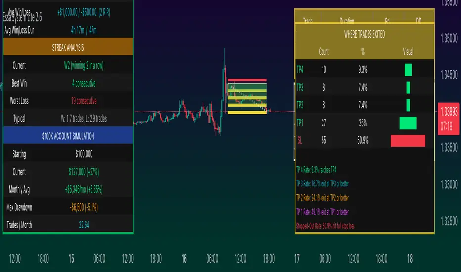
The Echo System🔊 The Echo System – Trend + Momentum Trading Strategy
Overview:
The Echo System is a trend-following and momentum-based trading tool designed to identify high-probability buy and sell signals through a combination of market trend analysis, price movement strength, and candlestick validation.
Key Features:
📈 Trend Detection:
Uses a 30 EMA vs. 200 EMA crossover to confirm bullish or bearish trends.
Visual trend strength meter powered by percentile ranking of EMA distance.
🔄 Momentum Check:
Detects significant price moves over the past 6 bars, enhanced by ATR-based scaling to filter weak signals.
🕯️ Candle Confirmation:
Validates recent price action using the previous and current candle body direction.
✅ Smart Conditions Table:
A live dashboard showing all trade condition checks (Trend, Recent Price Move, Candlestick confirmations) in real-time with visual feedback.
📊 Backtesting & Stats:
Auto-calculates average win, average loss, risk-reward ratio (RRR), and win rate across historical signals.
Clean performance dashboard with color-coded metrics for easy reading.
🔔 Alerts:
Set alerts for trade signals or significant price movements to stay updated without monitoring the chart 24/7.
Visuals:
Trend markers and price movement flags plotted directly on the chart.
Dual tables:
📈 Conditions table (top-right): breaks down trade criteria status.
📊 Performance table (bottom-right): shows real-time stats on win/loss and RRR.🔊 The Echo System – Trend + Momentum Trading Strategy
Overview:
The Echo System is a trend-following and momentum-based trading tool designed to identify high-probability buy and sell signals through a combination of market trend analysis, price movement strength, and candlestick validation.
Key Features:
📈 Trend Detection:
Uses a 30 EMA vs. 200 EMA crossover to confirm bullish or bearish trends.
Visual trend strength meter powered by percentile ranking of EMA distance.
🔄 Momentum Check:
Detects significant price moves over the past 6 bars, enhanced by ATR-based scaling to filter weak signals.
🕯️ Candle Confirmation:
Validates recent price action using the previous and current candle body direction.
✅ Smart Conditions Table:
A live dashboard showing all trade condition checks (Trend, Recent Price Move, Candlestick confirmations) in real-time with visual feedback.
📊 Backtesting & Stats:
Auto-calculates average win, average loss, risk-reward ratio (RRR), and win rate across historical signals.
Clean performance dashboard with color-coded metrics for easy reading.
🔔 Alerts:
Set alerts for trade signals or significant price movements to stay updated without monitoring the chart 24/7.
Visuals:
Trend markers and price movement flags plotted directly on the chart.
Dual tables:
📈 Conditions table (top-right): breaks down trade criteria status.
📊 Performance table (bottom-right): shows real-time stats on win/loss and RRR.
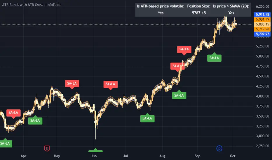
ATR Bands with ATR Cross + InfoTableOverview
This Pine Script™ indicator is designed to enhance traders' ability to analyze market volatility, trend direction, and position sizing directly on their TradingView charts. By plotting Average True Range (ATR) bands anchored at the OHLC4 price, displaying crossover labels, and providing a comprehensive information table, this tool offers a multifaceted approach to technical analysis.
Key Features:
ATR Bands Anchored at OHLC4: Visual representation of short-term and long-term volatility bands centered around the average price.
OHLC4 Dotted Line: A dotted line representing the average of Open, High, Low, and Close prices.
ATR Cross Labels: Visual cues indicating when short-term volatility exceeds long-term volatility and vice versa.
Information Table: Displays real-time data on market volatility, calculated position size based on risk parameters, and trend direction relative to the 20-period Smoothed Moving Average (SMMA).
Purpose
The primary purpose of this indicator is to:
Assess Market Volatility: By comparing short-term and long-term ATR values, traders can gauge the current volatility environment.
Determine Optimal Position Sizing: A calculated position size based on user-defined risk parameters helps in effective risk management.
Identify Trend Direction: Comparing the current price to the 20-period SMMA assists in determining the prevailing market trend.
Enhance Decision-Making: Visual cues and real-time data enable traders to make informed trading decisions with greater confidence.
How It Works
1. ATR Bands Anchored at OHLC4
Average True Range (ATR) Calculations
Short-Term ATR (SA): Calculated over a 9-period using ta.atr(9).
Long-Term ATR (LA): Calculated over a 21-period using ta.atr(21).
Plotting the Bands
OHLC4 Dotted Line: Plotted using small circles to simulate a dotted line due to Pine Script limitations.
ATR(9) Bands: Plotted in blue with semi-transparent shading.
ATR(21) Bands: Plotted in orange with semi-transparent shading.
Overlap: Bands can overlap, providing visual insights into changes in volatility.
2. ATR Cross Labels
Crossover Detection:
SA > LA: Indicates increasing short-term volatility.
Detected using ta.crossover(SA, LA).
A green upward label "SA>LA" is plotted below the bar.
SA < LA: Indicates decreasing short-term volatility.
Detected using ta.crossunder(SA, LA).
A red downward label "SA LA, then the market is considered volatile.
Display: Shows "Yes" or "No" based on the comparison.
b. Position Size Calculation
Risk Total Amount: User-defined input representing the total capital at risk.
Risk per 1 Stock: User-defined input representing the risk associated with one unit of the asset.
Purpose: Helps traders determine the appropriate position size based on their risk tolerance and current market volatility.
c. Is Price > 20 SMMA?
SMMA Calculation:
Calculated using a 20-period Smoothed Moving Average with ta.rma(close, 20).
Logic: If the current close price is above the SMMA, the trend is considered upward.
Display: Shows "Yes" or "No" based on the comparison.
How to Use
Step 1: Add the Indicator to Your Chart
Copy the Script: Copy the entire Pine Script code into the TradingView Pine Editor.
Save and Apply: Save the script and click "Add to Chart."
Step 2: Configure Inputs
Risk Parameters: Adjust the "Risk Total Amount" and "Risk per 1 Stock" in the indicator settings to match your personal risk management strategy.
Step 3: Interpret the Visuals
ATR Bands
Width of Bands: Wider bands indicate higher volatility; narrower bands indicate lower volatility.
Band Overlap: Pay attention to areas where the blue and orange bands diverge or converge.
OHLC4 Dotted Line
Serves as a central reference point for the ATR bands.
Helps visualize the average price around which volatility is measured.
ATR Cross Labels
"SA>LA" Label:
Indicates short-term volatility is increasing relative to long-term volatility.
May signal potential breakout or trend acceleration.
"SA 20 SMMA?
Use this to confirm trend direction before entering or exiting trades.
Practical Example
Imagine you are analyzing a stock and notice the following:
ATR(9) Crosses Above ATR(21):
A green "SA>LA" label appears.
The info table shows "Yes" for "Is ATR-based price volatile."
Position Size:
Based on your risk parameters, the position size is calculated.
Price Above 20 SMMA:
The info table shows "Yes" for "Is price > 20 SMMA."
Interpretation:
The market is experiencing increasing short-term volatility.
The trend is upward, as the price is above the 20 SMMA.
You may consider entering a long position, using the calculated position size to manage risk.
Customization
Colors and Transparency:
Adjust the colors of the bands and labels to suit your preferences.
Risk Parameters:
Modify the default values for risk amounts in the inputs.
Moving Average Period:
Change the SMMA period if desired.
Limitations and Considerations
Lagging Indicators: ATR and SMMA are lagging indicators and may not predict future price movements.
Market Conditions: The effectiveness of this indicator may vary across different assets and market conditions.
Risk of Overfitting: Relying solely on this indicator without considering other factors may lead to suboptimal trading decisions.
Conclusion
This indicator combines essential elements of technical analysis to provide a comprehensive tool for traders. By visualizing ATR bands anchored at the OHLC4, indicating volatility crossovers, and providing real-time data on position sizing and trend direction, it aids in making informed trading decisions.
Whether you're a novice trader looking to understand market volatility or an experienced trader seeking to refine your strategy, this indicator offers valuable insights directly on your TradingView charts.
Code Summary
The script is written in Pine Script™ version 5 and includes:
Calculations for OHLC4, ATRs, Bands, SMMA:
Uses built-in functions like ta.atr() and ta.rma() for calculations.
Plotting Functions:
plotshape() for the OHLC4 dotted line.
plot() and fill() for the ATR bands.
Crossover Detection:
ta.crossover() and ta.crossunder() for detecting ATR crosses.
Labeling Crossovers:
label.new() to place informative labels on the chart.
Information Table Creation:
table.new() to create the table.
table.cell() to populate it with data.
Acknowledgments
ATR and SMMA Concepts: Built upon standard technical analysis concepts widely used in trading.
Pine Script™: Leveraged the capabilities of Pine Script™ version 5 for advanced charting and analysis.
Note: Always test any indicator thoroughly and consider combining it with other forms of analysis before making trading decisions. Trading involves risk, and past performance is not indicative of future results.
Happy Trading!
RSI Overbought/Oversold + Divergence Indicator (new)//@version=5
indicator('CryptoSignalScanner - RSI Overbought/Oversold + Divergence Indicator (new)',
//---------------------------------------------------------------------------------------------------------------------------------
//--- Define Colors ---------------------------------------------------------------------------------------------------------------
//---------------------------------------------------------------------------------------------------------------------------------
vWhite = #FFFFFF
vViolet = #C77DF3
vIndigo = #8A2BE2
vBlue = #009CDF
vGreen = #5EBD3E
vYellow = #FFB900
vRed = #E23838
longColor = color.green
shortColor = color.red
textColor = color.white
bullishColor = color.rgb(38,166,154,0) //Used in the display table
bearishColor = color.rgb(239,83,79,0) //Used in the display table
nomatchColor = color.silver //Used in the display table
//---------------------------------------------------------------------------------------------------------------------------------------------------------------------
//--- Functions--------------------------------------------------------------------------------------------------------------------------------------------------------
//---------------------------------------------------------------------------------------------------------------------------------------------------------------------
TF2txt(TF) =>
switch TF
"S" => "RSI 1s:"
"5S" => "RSI 5s:"
"10S" => "RSI 10s:"
"15S" => "RSI 15s:"
"30S" => "RSI 30s"
"1" => "RSI 1m:"
"3" => "RSI 3m:"
"5" => "RSI 5m:"
"15" => "RSI 15m:"
"30" => "RSI 30m"
"45" => "RSI 45m"
"60" => "RSI 1h:"
"120" => "RSI 2h:"
"180" => "RSI 3h:"
"240" => "RSI 4h:"
"480" => "RSI 8h:"
"D" => "RSI 1D:"
"1D" => "RSI 1D:"
"2D" => "RSI 2D:"
"3D" => "RSI 2D:"
"3D" => "RSI 3W:"
"W" => "RSI 1W:"
"1W" => "RSI 1W:"
"M" => "RSI 1M:"
"1M" => "RSI 1M:"
"3M" => "RSI 3M:"
"6M" => "RSI 6M:"
"12M" => "RSI 12M:"
//---------------------------------------------------------------------------------------------------------------------------------------------------------------------
//--- Show/Hide Settings ----------------------------------------------------------------------------------------------------------------------------------------------
//---------------------------------------------------------------------------------------------------------------------------------------------------------------------
rsiShowInput = input(true, title='Show RSI', group='Show/Hide Settings')
maShowInput = input(false, title='Show MA', group='Show/Hide Settings')
showRSIMAInput = input(true, title='Show RSIMA Cloud', group='Show/Hide Settings')
rsiBandShowInput = input(true, title='Show Oversold/Overbought Lines', group='Show/Hide Settings')
rsiBandExtShowInput = input(true, title='Show Oversold/Overbought Extended Lines', group='Show/Hide Settings')
rsiHighlightShowInput = input(true, title='Show Oversold/Overbought Highlight Lines', group='Show/Hide Settings')
DivergenceShowInput = input(true, title='Show RSI Divergence Labels', group='Show/Hide Settings')
//---------------------------------------------------------------------------------------------------------------------------------------------------------------------
//--- Table Settings --------------------------------------------------------------------------------------------------------------------------------------------------
//---------------------------------------------------------------------------------------------------------------------------------------------------------------------
rsiShowTable = input(true, title='Show RSI Table Information box', group="RSI Table Settings")
rsiTablePosition = input.string(title='Location', defval='middle_right', options= , group="RSI Table Settings", inline='1')
rsiTextSize = input.string(title=' Size', defval='small', options= , group="RSI Table Settings", inline='1')
rsiShowTF1 = input(true, title='Show TimeFrame1', group="RSI Table Settings", inline='tf1')
rsiTF1 = input.timeframe("15", title=" Time", group="RSI Table Settings", inline='tf1')
rsiShowTF2 = input(true, title='Show TimeFrame2', group="RSI Table Settings", inline='tf2')
rsiTF2 = input.timeframe("60", title=" Time", group="RSI Table Settings", inline='tf2')
rsiShowTF3 = input(true, title='Show TimeFrame3', group="RSI Table Settings", inline='tf3')
rsiTF3 = input.timeframe("240", title=" Time", group="RSI Table Settings", inline='tf3')
rsiShowTF4 = input(true, title='Show TimeFrame4', group="RSI Table Settings", inline='tf4')
rsiTF4 = input.timeframe("D", title=" Time", group="RSI Table Settings", inline='tf4')
rsiShowHist = input(true, title='Show RSI Historical Columns', group="RSI Table Settings", tooltip='Show the information of the 2 previous closed candles')
//---------------------------------------------------------------------------------------------------------------------------------------------------------------------
//--- RSI Input Settings ----------------------------------------------------------------------------------------------------------------------------------------------
//---------------------------------------------------------------------------------------------------------------------------------------------------------------------
rsiSourceInput = input.source(close, 'Source', group='RSI Settings')
rsiLengthInput = input.int(14, minval=1, title='RSI Length', group='RSI Settings', tooltip='Here we set the RSI lenght')
rsiColorInput = input.color(#26a69a, title="RSI Color", group='RSI Settings')
rsimaColorInput = input.color(#ef534f, title="RSIMA Color", group='RSI Settings')
rsiBandColorInput = input.color(#787B86, title="RSI Band Color", group='RSI Settings')
rsiUpperBandExtInput = input.int(title='RSI Overbought Extended Line', defval=80, minval=50, maxval=100, group='RSI Settings')
rsiUpperBandInput = input.int(title='RSI Overbought Line', defval=70, minval=50, maxval=100, group='RSI Settings')
rsiLowerBandInput = input.int(title='RSI Oversold Line', defval=30, minval=0, maxval=50, group='RSI Settings')
rsiLowerBandExtInput = input.int(title='RSI Oversold Extended Line', defval=20, minval=0, maxval=50, group='RSI Settings')
//---------------------------------------------------------------------------------------------------------------------------------------------------------------------
//--- MA Input Settings -----------------------------------------------------------------------------------------------------------------------------------------------
//---------------------------------------------------------------------------------------------------------------------------------------------------------------------
maTypeInput = input.string("EMA", title="MA Type", options= , group="MA Settings")
maLengthInput = input.int(14, title="MA Length", group="MA Settings")
maColorInput = input.color(color.yellow, title="MA Color", group='MA Settings') //#7E57C2
//---------------------------------------------------------------------------------------------------------------------------------------------------------------------
//--- Divergence Input Settings ---------------------------------------------------------------------------------------------------------------------------------------
//---------------------------------------------------------------------------------------------------------------------------------------------------------------------
lbrInput = input(title="Pivot Lookback Right", defval=2, group='RSI Divergence Settings')
lblInput = input(title="Pivot Lookback Left", defval=2, group='RSI Divergence Settings')
lbRangeMaxInput = input(title="Max of Lookback Range", defval=10, group='RSI Divergence Settings')
lbRangeMinInput = input(title="Min of Lookback Range", defval=2, group='RSI Divergence Settings')
plotBullInput = input(title="Plot Bullish", defval=true, group='RSI Divergence Settings')
plotHiddenBullInput = input(title="Plot Hidden Bullish", defval=true, group='RSI Divergence Settings')
plotBearInput = input(title="Plot Bearish", defval=true, group='RSI Divergence Settings')
plotHiddenBearInput = input(title="Plot Hidden Bearish", defval=true, group='RSI Divergence Settings')
//---------------------------------------------------------------------------------------------------------------------------------------------------------------------
//--- RSI Calculation -------------------------------------------------------------------------------------------------------------------------------------------------
//---------------------------------------------------------------------------------------------------------------------------------------------------------------------
rsi = ta.rsi(rsiSourceInput, rsiLengthInput)
rsiprevious = rsi
= request.security(syminfo.tickerid, rsiTF1, [rsi, rsi , rsi ], lookahead=barmerge.lookahead_on)
= request.security(syminfo.tickerid, rsiTF2, [rsi, rsi , rsi ], lookahead=barmerge.lookahead_on)
= request.security(syminfo.tickerid, rsiTF3, [rsi, rsi , rsi ], lookahead=barmerge.lookahead_on)
= request.security(syminfo.tickerid, rsiTF4, [rsi, rsi , rsi ], lookahead=barmerge.lookahead_on)
//---------------------------------------------------------------------------------------------------------------------------------------------------------------------
//--- MA Calculation -------------------------------------------------------------------------------------------------------------------------------------------------
//---------------------------------------------------------------------------------------------------------------------------------------------------------------------
ma(source, length, type) =>
switch type
"SMA" => ta.sma(source, length)
"Bollinger Bands" => ta.sma(source, length)
"EMA" => ta.ema(source, length)
"SMMA (RMA)" => ta.rma(source, length)
"WMA" => ta.wma(source, length)
"VWMA" => ta.vwma(source, length)
rsiMA = ma(rsi, maLengthInput, maTypeInput)
rsiMAPrevious = rsiMA
//---------------------------------------------------------------------------------------------------------------------------------------------------------------------
//--- Stoch RSI Settings + Calculation --------------------------------------------------------------------------------------------------------------------------------
//---------------------------------------------------------------------------------------------------------------------------------------------------------------------
showStochRSI = input(false, title="Show Stochastic RSI", group='Stochastic RSI Settings')
smoothK = input.int(title="Stochastic K", defval=3, minval=1, maxval=10, group='Stochastic RSI Settings')
smoothD = input.int(title="Stochastic D", defval=4, minval=1, maxval=10, group='Stochastic RSI Settings')
lengthRSI = input.int(title="Stochastic RSI Lenght", defval=14, minval=1, group='Stochastic RSI Settings')
lengthStoch = input.int(title="Stochastic Lenght", defval=14, minval=1, group='Stochastic RSI Settings')
colorK = input.color(color.rgb(41,98,255,0), title="K Color", group='Stochastic RSI Settings', inline="1")
colorD = input.color(color.rgb(205,109,0,0), title="D Color", group='Stochastic RSI Settings', inline="1")
StochRSI = ta.rsi(rsiSourceInput, lengthRSI)
k = ta.sma(ta.stoch(StochRSI, StochRSI, StochRSI, lengthStoch), smoothK) //Blue Line
d = ta.sma(k, smoothD) //Red Line
//---------------------------------------------------------------------------------------------------------------------------------------------------------------------
//--- Divergence Settings ------------------------------------------------------------------------------------------------------------------------------------------
//---------------------------------------------------------------------------------------------------------------------------------------------------------------------
bearColor = color.red
bullColor = color.green
hiddenBullColor = color.new(color.green, 50)
hiddenBearColor = color.new(color.red, 50)
//textColor = color.white
noneColor = color.new(color.white, 100)
osc = rsi
plFound = na(ta.pivotlow(osc, lblInput, lbrInput)) ? false : true
phFound = na(ta.pivothigh(osc, lblInput, lbrInput)) ? false : true
_inRange(cond) =>
bars = ta.barssince(cond == true)
lbRangeMinInput <= bars and bars <= lbRangeMaxInput
//---------------------------------------------------------------------------------------------------------------------------------------------------------------------
//--- Define Plot & Line Colors ---------------------------------------------------------------------------------------------------------------------------------------
//---------------------------------------------------------------------------------------------------------------------------------------------------------------------
rsiColor = rsi >= rsiMA ? rsiColorInput : rsimaColorInput
//---------------------------------------------------------------------------------------------------------------------------------------------------------------------
//--- Plot Lines ------------------------------------------------------------------------------------------------------------------------------------------------------
//---------------------------------------------------------------------------------------------------------------------------------------------------------------------
// Create a horizontal line at a specific price level
myLine = line.new(bar_index , 75, bar_index, 75, color = color.rgb(187, 14, 14), width = 2)
bottom = line.new(bar_index , 50, bar_index, 50, color = color.rgb(223, 226, 28), width = 2)
mymainLine = line.new(bar_index , 60, bar_index, 60, color = color.rgb(13, 154, 10), width = 3)
hline(50, title='RSI Baseline', color=color.new(rsiBandColorInput, 50), linestyle=hline.style_solid, editable=false)
hline(rsiBandExtShowInput ? rsiUpperBandExtInput : na, title='RSI Upper Band', color=color.new(rsiBandColorInput, 10), linestyle=hline.style_dashed, editable=false)
hline(rsiBandShowInput ? rsiUpperBandInput : na, title='RSI Upper Band', color=color.new(rsiBandColorInput, 10), linestyle=hline.style_dashed, editable=false)
hline(rsiBandShowInput ? rsiLowerBandInput : na, title='RSI Upper Band', color=color.new(rsiBandColorInput, 10), linestyle=hline.style_dashed, editable=false)
hline(rsiBandExtShowInput ? rsiLowerBandExtInput : na, title='RSI Upper Band', color=color.new(rsiBandColorInput, 10), linestyle=hline.style_dashed, editable=false)
bgcolor(rsiHighlightShowInput ? rsi >= rsiUpperBandExtInput ? color.new(rsiColorInput, 70) : na : na, title="Show Extended Oversold Highlight", editable=false)
bgcolor(rsiHighlightShowInput ? rsi >= rsiUpperBandInput ? rsi < rsiUpperBandExtInput ? color.new(#64ffda, 90) : na : na: na, title="Show Overbought Highlight", editable=false)
bgcolor(rsiHighlightShowInput ? rsi <= rsiLowerBandInput ? rsi > rsiLowerBandExtInput ? color.new(#F43E32, 90) : na : na : na, title="Show Extended Oversold Highlight", editable=false)
bgcolor(rsiHighlightShowInput ? rsi <= rsiLowerBandInput ? color.new(rsimaColorInput, 70) : na : na, title="Show Oversold Highlight", editable=false)
maPlot = plot(maShowInput ? rsiMA : na, title='MA', color=color.new(maColorInput,0), linewidth=1)
rsiMAPlot = plot(showRSIMAInput ? rsiMA : na, title="RSI EMA", color=color.new(rsimaColorInput,0), editable=false, display=display.none)
rsiPlot = plot(rsiShowInput ? rsi : na, title='RSI', color=color.new(rsiColor,0), linewidth=1)
fill(rsiPlot, rsiMAPlot, color=color.new(rsiColor, 60), title="RSIMA Cloud")
plot(showStochRSI ? k : na, title='Stochastic K', color=colorK, linewidth=1)
plot(showStochRSI ? d : na, title='Stochastic D', color=colorD, linewidth=1)
//---------------------------------------------------------------------------------------------------------------------------------------------------------------------
//--- Plot Divergence -------------------------------------------------------------------------------------------------------------------------------------------------
//---------------------------------------------------------------------------------------------------------------------------------------------------------------------
// Regular Bullish
// Osc: Higher Low
oscHL = osc > ta.valuewhen(plFound, osc , 1) and _inRange(plFound )
// Price: Lower Low
priceLL = low < ta.valuewhen(plFound, low , 1)
bullCond = plotBullInput and priceLL and oscHL and plFound
plot(
plFound ? osc : na,
offset=-lbrInput,
title="Regular Bullish",
linewidth=2,
color=(bullCond ? bullColor : noneColor)
)
plotshape(
DivergenceShowInput ? bullCond ? osc : na : na,
offset=-lbrInput,
title="Regular Bullish Label",
text=" Bull ",
style=shape.labelup,
location=location.absolute,
color=bullColor,
textcolor=textColor
)
//------------------------------------------------------------------------------
// Hidden Bullish
// Osc: Lower Low
oscLL = osc < ta.valuewhen(plFound, osc , 1) and _inRange(plFound )
// Price: Higher Low
priceHL = low > ta.valuewhen(plFound, low , 1)
hiddenBullCond = plotHiddenBullInput and priceHL and oscLL and plFound
plot(
plFound ? osc : na,
offset=-lbrInput,
title="Hidden Bullish",
linewidth=2,
color=(hiddenBullCond ? hiddenBullColor : noneColor)
)
plotshape(
DivergenceShowInput ? hiddenBullCond ? osc : na : na,
offset=-lbrInput,
title="Hidden Bullish Label",
text=" H Bull ",
style=shape.labelup,
location=location.absolute,
color=bullColor,
textcolor=textColor
)
//------------------------------------------------------------------------------
// Regular Bearish
// Osc: Lower High
oscLH = osc < ta.valuewhen(phFound, osc , 1) and _inRange(phFound )
// Price: Higher High
priceHH = high > ta.valuewhen(phFound, high , 1)
bearCond = plotBearInput and priceHH and oscLH and phFound
plot(
phFound ? osc : na,
offset=-lbrInput,
title="Regular Bearish",
linewidth=2,
color=(bearCond ? bearColor : noneColor)
)
plotshape(
DivergenceShowInput ? bearCond ? osc : na : na,
offset=-lbrInput,
title="Regular Bearish Label",
text=" Bear ",
style=shape.labeldown,
location=location.absolute,
color=bearColor,
textcolor=textColor
)
//------------------------------------------------------------------------------
// Hidden Bearish
// Osc: Higher High
oscHH = osc > ta.valuewhen(phFound, osc , 1) and _inRange(phFound )
// Price: Lower High
priceLH = high < ta.valuewhen(phFound, high , 1)
hiddenBearCond = plotHiddenBearInput and priceLH and oscHH and phFound
plot(
phFound ? osc : na,
offset=-lbrInput,
title="Hidden Bearish",
linewidth=2,
color=(hiddenBearCond ? hiddenBearColor : noneColor)
)
plotshape(
DivergenceShowInput ? hiddenBearCond ? osc : na : na,
offset=-lbrInput,
title="Hidden Bearish Label",
text=" H Bear ",
style=shape.labeldown,
location=location.absolute,
color=bearColor,
textcolor=textColor
)
//---------------------------------------------------------------------------------------------------------------------------------------------------------------------
//--- Check RSI Lineup ------------------------------------------------------------------------------------------------------------------------------------------------
//---------------------------------------------------------------------------------------------------------------------------------------------------------------------
bullTF = rsi > rsi and rsi > rsi
bearTF = rsi < rsi and rsi < rsi
bullTF1 = rsi1 > rsi1_1 and rsi1_1 > rsi1_2
bearTF1 = rsi1 < rsi1_1 and rsi1_1 < rsi1_2
bullTF2 = rsi2 > rsi2_1 and rsi2_1 > rsi2_2
bearTF2 = rsi2 < rsi2_1 and rsi2_1 < rsi2_2
bullTF3 = rsi3 > rsi3_1 and rsi3_1 > rsi3_2
bearTF3 = rsi3 < rsi3_1 and rsi3_1 < rsi3_2
bullTF4 = rsi4 > rsi4_1 and rsi4_1 > rsi4_2
bearTF4 = rsi4 < rsi4_1 and rsi4_1 < rsi4_2
bbTxt(bull,bear) =>
bull ? "BULLISH" : bear ? "BEARISCH" : 'NO LINEUP'
bbColor(bull,bear) =>
bull ? bullishColor : bear ? bearishColor : nomatchColor
newTC(tBox, col, row, txt, width, txtColor, bgColor, txtHA, txtSize) =>
table.cell(table_id=tBox,column=col, row=row, text=txt, width=width,text_color=txtColor,bgcolor=bgColor, text_halign=txtHA, text_size=txtSize)
//---------------------------------------------------------------------------------------------------------------------------------------------------------------------
//--- Define RSI Table Setting ----------------------------------------------------------------------------------------------------------------------------------------
//---------------------------------------------------------------------------------------------------------------------------------------------------------------------
width_c0 = 0
width_c1 = 0
if rsiShowTable
var tBox = table.new(position=rsiTablePosition, columns=5, rows=6, bgcolor=color.rgb(18,22,33,50), frame_color=color.black, frame_width=1, border_color=color.black, border_width=1)
newTC(tBox, 0,1,"RSI Current",width_c0,color.orange,color.rgb(0,0,0,100),'right',rsiTextSize)
newTC(tBox, 1,1,str.format(" {0,number,#.##} ", rsi),width_c0,vWhite,rsi < 50 ? bearishColor:bullishColor,'left',rsiTextSize)
newTC(tBox, 4,1,bbTxt(bullTF, bearTF),width_c0,vWhite,bbColor(bullTF, bearTF),'center',rsiTextSize)
if rsiShowHist
newTC(tBox, 2,1,str.format(" {0,number,#.##} ", rsi ),width_c0,vWhite,rsi < 50 ? bearishColor:bullishColor,'left',rsiTextSize)
newTC(tBox, 3,1,str.format(" {0,number,#.##} ", rsi ),width_c0,vWhite,rsi < 50 ? bearishColor:bullishColor,'left',rsiTextSize)
if rsiShowTF1
newTC(tBox, 0,2,TF2txt(rsiTF1),width_c0,vWhite,color.rgb(0,0,0,100),'right',rsiTextSize)
newTC(tBox, 1,2,str.format(" {0,number,#.##} ", rsi1),width_c0,vWhite,rsi1 < 50 ? bearishColor:bullishColor,'left',rsiTextSize)
newTC(tBox, 4,2,bbTxt(bullTF1, bearTF1),width_c0,vWhite,bbColor(bullTF1,bearTF1),'center',rsiTextSize)
if rsiShowHist
newTC(tBox, 2,2,str.format(" {0,number,#.##} ", rsi1_1),width_c0,vWhite,rsi1_1 < 50 ? bearishColor:bullishColor,'left',rsiTextSize)
newTC(tBox, 3,2,str.format(" {0,number,#.##} ", rsi1_2),width_c0,vWhite,rsi1_2 < 50 ? bearishColor:bullishColor,'left',rsiTextSize)
if rsiShowTF2
newTC(tBox, 0,3,TF2txt(rsiTF2),width_c0,vWhite,color.rgb(0,0,0,100),'right',rsiTextSize)
newTC(tBox, 1,3,str.format(" {0,number,#.##} ", rsi2),width_c0,vWhite,rsi2 < 50 ? bearishColor:bullishColor,'left',rsiTextSize)
newTC(tBox, 4,3,bbTxt(bullTF2, bearTF2),width_c0,vWhite,bbColor(bullTF2,bearTF2),'center',rsiTextSize)
if rsiShowHist
newTC(tBox, 2,3,str.format(" {0,number,#.##} ", rsi2_1),width_c0,vWhite,rsi2_1 < 50 ? bearishColor:bullishColor,'left',rsiTextSize)
newTC(tBox, 3,3,str.format(" {0,number,#.##} ", rsi2_2),width_c0,vWhite,rsi2_2 < 50 ? bearishColor:bullishColor,'left',rsiTextSize)
if rsiShowTF3
newTC(tBox, 0,4,TF2txt(rsiTF3),width_c0,vWhite,color.rgb(0,0,0,100),'right',rsiTextSize)
newTC(tBox, 1,4,str.format(" {0,number,#.##} ", rsi3),width_c0,vWhite,rsi3 < 50 ? bearishColor:bullishColor,'left',rsiTextSize)
newTC(tBox, 4,4,bbTxt(bullTF3, bearTF3),width_c0,vWhite,bbColor(bullTF3,bearTF3),'center',rsiTextSize)
if rsiShowHist
newTC(tBox, 2,4,str.format(" {0,number,#.##} ", rsi3_1),width_c0,vWhite,rsi3_1 < 50 ? bearishColor:bullishColor,'left',rsiTextSize)
newTC(tBox, 3,4,str.format(" {0,number,#.##} ", rsi3_2),width_c0,vWhite,rsi3_2 < 50 ? bearishColor:bullishColor,'left',rsiTextSize)
if rsiShowTF4
newTC(tBox, 0,5,TF2txt(rsiTF4),width_c0,vWhite,color.rgb(0,0,0,100),'right',rsiTextSize)
newTC(tBox, 1,5,str.format(" {0,number,#.##} ", rsi4),width_c0,vWhite,rsi4 < 50 ? bearishColor:bullishColor,'left',rsiTextSize)
newTC(tBox, 4,5,bbTxt(bullTF4, bearTF4),width_c0,vWhite,bbColor(bullTF4,bearTF4),'center',rsiTextSize)
if rsiShowHist
newTC(tBox, 2,5,str.format(" {0,number,#.##} ", rsi4_1),width_c0,vWhite,rsi4_1 < 50 ? bearishColor:bullishColor,'left',rsiTextSize)
newTC(tBox, 3,5,str.format(" {0,number,#.##} ", rsi4_2),width_c0,vWhite,rsi4_2 < 50 ? bearishColor:bullishColor,'left',rsiTextSize)
//------------------------------------------------------
//--- Alerts -------------------------------------------
//------------------------------------------------------

Triad Trade MatrixOverview
Triad Trade Matrix is an advanced multi-strategy indicator built using Pine Script v5. It is designed to simultaneously track and display key trading metrics for three distinct trading styles on a single chart:
Swing Trading (Swing Supreme):
This mode captures longer-term trends and is designed for trades that typically span several days. It uses customizable depth and deviation parameters to determine swing signals.
Day Trading (Day Blaze):
This mode focuses on intraday price movements. It generates signals that are intended to be executed within a single trading session. The parameters for depth and deviation are tuned to capture more frequent, shorter-term moves.
Scalping (Scalp Surge):
This mode is designed for very short-term trades where quick entries and exits are key. It uses more sensitive parameters to detect rapid price movements suitable for scalping strategies.
Each trading style is represented by its own merged table that displays real-time metrics. The tables update automatically as new trading signals are generated.
Key Features
Multi-Style Tracking:
Swing Supreme (Large): For swing trading; uses a purple theme.
Day Blaze (Medium): For day trading; uses an orange theme.
Scalp Surge (Small): For scalping; uses a green theme.
Real-Time Metrics:
Each table displays key trade metrics including:
Entry Price: The price at which the trade was entered.
Exit Price: The price at which the previous trade was exited.
Position Size: Calculated as the account size divided by the entry price.
Direction: Indicates whether the trade is “Up” (long) or “Down” (short).
Time: The time when the trade was executed (formatted to hours and minutes).
Wins/Losses: The cumulative number of winning and losing trades.
Current Price & PnL: The current price on the chart and the profit/loss computed relative to the entry price.
Duration: The number of bars that the trade has been open.
History Column: A merged summary column that shows the most recent trade’s details (entry, exit, and result).
Customizability:
Column Visibility: Users can toggle individual columns (Ticker, Timeframe, Entry, Exit, etc.) on or off according to their preference.
Appearance Settings: You can customize the table border width, frame color, header background, and text colors.
History Toggle: The merged history column can be enabled or disabled.
Chart Markers: There is an option to show or hide chart markers (labels and lines) that indicate trade entries and exits on the chart.
Trade History Management:
The indicator maintains a rolling history (up to three recent trades per trading style) and displays the latest summary in the merged table.
This history column provides a quick reference to recent performance.
How It Works
Signal Generation & Trade Metrics
Trade Entry/Exit Calculation:
For each trading style, the indicator uses built-in functions (such as ta.lowestbars and ta.highestbars) to analyze price movements. Based on a customizable "depth" and "deviation" parameter, it determines the point of entry for a trade.
Swing Supreme: Uses larger depth/deviation values to capture swing trends.
Day Blaze: Uses intermediate values for intraday moves.
Scalp Surge: Uses tighter parameters to pick up rapid price changes.
Metrics Update:
When a new trade signal is generated (i.e., when the trade entry price is updated), the indicator calculates:
The current PnL as the difference between the current price and the entry price (or vice versa, depending on the trade direction).
The duration as the number of bars since the trade was opened.
The position size using the formula: accountSize / entryPrice.
History Recording:
Each time a new trade is triggered (i.e., when the entry price is updated), a summary string is created (showing entry, exit, and win/loss status) and appended to the corresponding trade history array. The merged table then displays the latest summary from this history.
Table Display
Merged Table Structure:
Each trading style (Swing Supreme, Day Blaze, and Scalp Surge) is represented by a table that has 15 columns. The columns are:
Trade Type (e.g., Swing Supreme)
Ticker
Timeframe
Entry Price
Exit Price
Position Size
Direction
Time of Entry
Account Size
Wins
Losses
Current Price
Current PnL
Duration (in bars)
History (the latest trade summary)
User Customization:
Through the settings panel, users can choose which columns to display.
If a column is toggled off, its cells will remain blank, allowing traders to focus on the metrics that matter most to them.
Appearance & Themes:
The table headers and cell backgrounds are customizable via color inputs. The trading style names are color-coded:
Swing Supreme (Large): Uses a purple theme.
Day Blaze (Medium): Uses an orange theme.
Scalp Surge (Small): Uses a green theme.
How to Use the Indicator
Add the Indicator to Your Chart:
Once published, add "Triad Trade Matrix" to your TradingView chart.
Configure the Settings:
Adjust the Account Size to match your trading capital.
Use the Depth and Deviation inputs for each trading style to fine-tune the signal sensitivity.
Toggle the Chart Markers on if you want visual entry/exit markers on the chart.
Customize which columns are visible via the column visibility toggles.
Enable or disable the History Column to show the merged trade history in the table.
Adjust the appearance settings (colors, border width, etc.) to suit your chart background and preferences.
Interpret the Tables:
Swing Supreme:
This table shows metrics for swing trades.
Look for changes in entry price, PnL, and trade duration to monitor longer-term moves.
Day Blaze:
This table tracks day trading activity.It will update more frequently, reflecting intraday trends.
Scalp Surge:
This table is dedicated to scalping signals.Use it to see quick entry/exit data and rapid profit/loss changes.
The History column (if enabled) gives you a snapshot of the most recent trade (e.g., "E:123.45 X:124.00 Up Win").
Use allerts:
The indicator includes alert condition for new trade entries(both long and short)for each trading style.
Summary:
Triad Trade Matrix provides an robust,multi-dimensional view of your trading performance across swing trading, day trading, and scalping.
Best to be used whith my other indicators
True low high
Vma Ext_Adv_CustomTbl
This indicator is ideal for traders who wish to monitor multiple trading styles simultaneously, with a clear, technical, and real-time display of performance metrics.
Happy Trading!

Argentum Flag [AGP] Ver.2.5Central Purpose and Concept
The Argentum Flag script is a multifunctional tool that integrates and visualizes multiple key indicators to provide a detailed and unified perspective of the market. The core concept is to analyze price from different angles—volatility, volume, and momentum—to identify confluences and patterns that may be difficult to see with separate indicators. This "mashup" is not a simple fusion of indicators, but a strategic combination of tools that complement each other to offer a comprehensive view of asset behavior.
Components and Their Functionality
This script combines and visualizes the following elements:
EMA Percentage Bands (EMA Bands):
Uses an Exponential Moving Average (EMA) as a baseline.
Calculates and draws several volatility bands that deviate from the central EMA by fixed percentages (0.47%, 0.94%, 2.36%). These bands are inspired by Fibonacci ratios and the cyclical nature of the market.
The bands are colored with a dynamic gradient that reflects the current state of volatility.
Utility: These bands act as dynamic support and resistance areas. The price entering or exiting these zones can indicate a change in volatility or a possible exhaustion of the movement.
Volatility Signals (Vortex & Prime Signals):
The script generates visual signals when the price stays outside the volatility bands for a specific number of bars.
Vortex Signals (diamond ⍲): Appear when the price crosses and stays outside the Prime bands, suggesting a high volatility or a possible continuation of the trend.
Exit/Entry Signals (circle ⌾): Are activated when the price stays outside the Vortex bands, indicating an extreme extension of volatility. These can be interpreted as potential reversal or profit-taking zones.
Utility: They help traders quickly identify moments of high and low volatility and potential turning points in price action.
Volume Analysis (Volume Bar Colors):
The script changes the color of the bars based on the relationship between the current volume and the average volume over a 50-bar period.
Utility: This feature allows the trader to immediately visualize the strength behind a price movement. For example, a bullish candle with "extreme" volume suggests strong buying interest, while a bearish candle with "low" volume could indicate a weak correction.
Summary Tables (Dashboard):
EMA-Fibo Table: Displays the values of 12 EMAs based on the Fibonacci sequence (5, 8, 13, 21...) in an easy-to-access table. The background color of each value indicates if the current price is above (bullish) or below (bearish) that EMA.
Multi-Timeframe RSI Table: Displays the Relative Strength Index (RSI) values across multiple timeframes (from 1 minute to monthly). The text color changes to highlight if the RSI is in overbought (orange) or oversold (white) areas, according to the established levels.
Utility: These tables condense a large amount of data into a simple format, allowing traders to perform a quick, multi-timeframe market analysis without constantly switching charts.
How to Use the Script
This script is a contextual analysis tool that works best when its different components are combined. It is not a "buy and sell signal" system on its own, but a tool for informed decision-making.
Trend Identification: Use the EMA table to see the general trend direction across different timeframes. A price above most of the EMAs in the table suggests a bullish bias.
Volatility Reading: Observe the EMA bands. If the price stays within the bands, volatility is low. A strong move that breaks out of the bands, accompanied by an "extreme" volume color (blue), suggests strong momentum that could continue.
Momentum Analysis: Use the RSI table to confirm movements. An overbought 15m RSI could support a reversal signal from the Vortex bands, while a 1D RSI in a neutral zone may indicate that the main trend has not changed.
Signal Confirmation: Visual signals (diamond and circle) should not be used in isolation. They must be confirmed by volume analysis and dashboard readings. For example, an "Exit Signal" (circle) with low volume may be less reliable than one with high volume and a clear reversal candle.
Disclaimer
This script is for informational and educational purposes only. It is not financial advice, nor is it a recommendation to buy or sell any financial instrument. All trading involves risk, and past performance is not indicative of future results. The user is solely responsible for their own trading decisions.

Relative Strength and MomentumRelative Strength and Momentum Indicator
Unlock deeper market insights with the Relative Strength and Momentum Indicator—a powerful tool designed to help traders and investors identify the strongest stocks and sectors based on relative performance. This custom indicator displays essential information on relative strength and momentum for up to 15 different symbols, compared against a benchmark index, all within a clear and organized table format.
Key Features:
1. Customizable Inputs: Choose up to 15 symbols to compare, along with a benchmark index, allowing you to tailor the indicator to your trading strategy. The 'Lookback Period' input defines how many weeks of data are analyzed for relative strength and momentum.
2. Relative Strength Calculation: For each selected symbol, the indicator calculates the Relative Strength (RS) against the chosen benchmark. This RS is further refined using an exponential moving average (EMA) to smooth the results, providing a more stable trend overview.
3. Momentum Analysis: Momentum is determined by analyzing the rate of change in relative strength. The indicator calculates a momentum rank for each symbol, based on its relative strength’s improvement or deterioration.
4. Percentile Ranking System: Each symbol is assigned a percentile rank (from 1 to 100) based on its relative strength compared to the others. Similarly, momentum rankings are also assigned from 1 to 100, offering a clear understanding of which assets are outperforming or underperforming.
5. Visual Indicators:
a. Green: Signals improving or stable relative strength and momentum.
b. Red: Indicates declining relative strength or momentum.
c. Aqua: Highlights symbols performing well on both relative strength and momentum—ideal candidates for further analysis.
6. Two Clear Tables:
a. Relative Strength Rank Table: Displays weekly rankings of relative strength for each symbol.
b. Momentum Table: Shows momentum trends, helping you identify which symbols are gaining or losing strength.
7. Color-Coded for Easy Analysis: The tables are color-coded to make analysis quick and straightforward. A green color means the symbol is performing well in terms of relative strength or momentum, while red indicates weaker performance. Aqua marks symbols that are excelling in both areas.
Use Case:
a. Sector Comparison: Identify which sectors or indexes are showing both relative strength and momentum to pick high-potential stocks. This allows you to align with broader market trends for improved trade entries.
b. Stock Selection: Quickly compare symbols within the same sector to find the stronger performers.
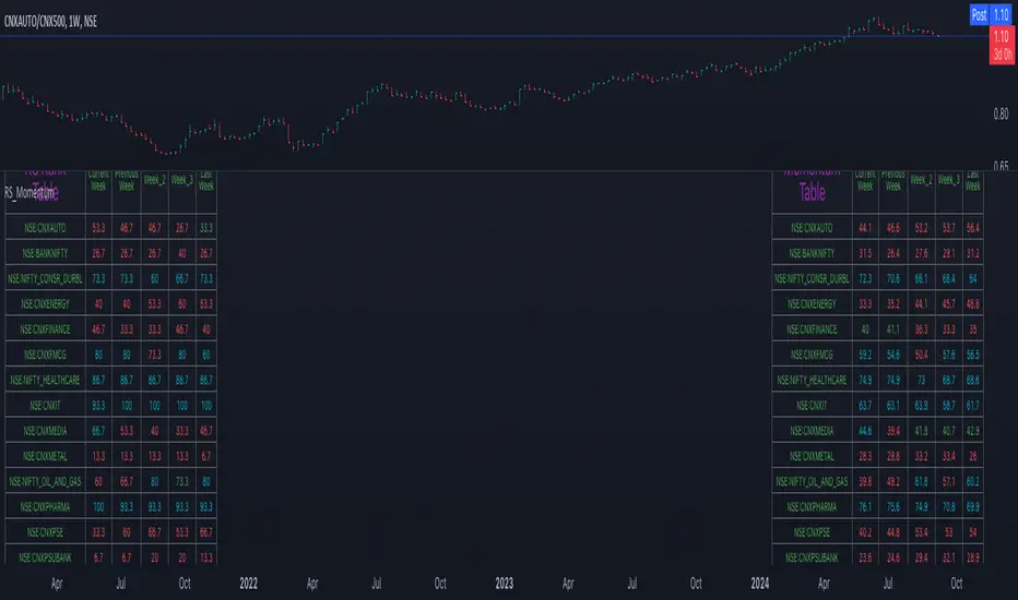
analytics_tablesLibrary "analytics_tables"
📝 Description
This library provides the implementation of several performance-related statistics and metrics, presented in the form of tables.
The metrics shown in the afforementioned tables where developed during the past years of my in-depth analalysis of various strategies in an atempt to reason about the performance of each strategy.
The visualization and some statistics where inspired by the existing implementations of the "Seasonality" script, and the performance matrix implementations of @QuantNomad and @ZenAndTheArtOfTrading scripts.
While this library is meant to be used by my strategy framework "Template Trailing Strategy (Backtester)" script, I wrapped it in a library hoping this can be usefull for other community strategy scripts that will be released in the future.
🤔 How to Guide
To use the functionality this library provides in your script you have to import it first!
Copy the import statement of the latest release by pressing the copy button below and then paste it into your script. Give a short name to this library so you can refer to it later on. The import statement should look like this:
import jason5480/analytics_tables/1 as ant
There are three types of tables provided by this library in the initial release. The stats table the metrics table and the seasonality table.
Each one shows different kinds of performance statistics.
The table UDT shall be initialized once using the `init()` method.
They can be updated using the `update()` method where the updated data UDT object shall be passed.
The data UDT can also initialized and get updated on demend depending on the use case
A code example for the StatsTable is the following:
var ant.StatsData statsData = ant.StatsData.new()
statsData.update(SideStats.new(), SideStats.new(), 0)
if (barstate.islastconfirmedhistory or (barstate.isrealtime and barstate.isconfirmed))
var statsTable = ant.StatsTable.new().init(ant.getTablePos('TOP', 'RIGHT'))
statsTable.update(statsData)
A code example for the MetricsTable is the following:
var ant.StatsData statsData = ant.StatsData.new()
statsData.update(ant.SideStats.new(), ant.SideStats.new(), 0)
if (barstate.islastconfirmedhistory or (barstate.isrealtime and barstate.isconfirmed))
var metricsTable = ant.MetricsTable.new().init(ant.getTablePos('BOTTOM', 'RIGHT'))
metricsTable.update(statsData, 10)
A code example for the SeasonalityTable is the following:
var ant.SeasonalData seasonalData = ant.SeasonalData.new().init(Seasonality.monthOfYear)
seasonalData.update()
if (barstate.islastconfirmedhistory or (barstate.isrealtime and barstate.isconfirmed))
var seasonalTable = ant.SeasonalTable.new().init(seasonalData, ant.getTablePos('BOTTOM', 'LEFT'))
seasonalTable.update(seasonalData)
🏋️♂️ Please refer to the "EXAMPLE" regions of the script for more advanced and up to date code examples!
Special thanks to @Mrcrbw for the proposal to develop this library and @DCNeu for the constructive feedback 🏆.
getTablePos(ypos, xpos)
Get table position compatible string
Parameters:
ypos (simple string) : The position on y axise
xpos (simple string) : The position on x axise
Returns: The position to be passed to the table
method init(this, pos, height, width, positiveTxtColor, negativeTxtColor, neutralTxtColor, positiveBgColor, negativeBgColor, neutralBgColor)
Initialize the stats table object with the given colors in the given position
Namespace types: StatsTable
Parameters:
this (StatsTable) : The stats table object
pos (simple string) : The table position string
height (simple float) : The height of the table as a percentage of the charts height. By default, 0 auto-adjusts the height based on the text inside the cells
width (simple float) : The width of the table as a percentage of the charts height. By default, 0 auto-adjusts the width based on the text inside the cells
positiveTxtColor (simple color) : The text color when positive
negativeTxtColor (simple color) : The text color when negative
neutralTxtColor (simple color) : The text color when neutral
positiveBgColor (simple color) : The background color with transparency when positive
negativeBgColor (simple color) : The background color with transparency when negative
neutralBgColor (simple color) : The background color with transparency when neutral
method init(this, pos, height, width, neutralBgColor)
Initialize the metrics table object with the given colors in the given position
Namespace types: MetricsTable
Parameters:
this (MetricsTable) : The metrics table object
pos (simple string) : The table position string
height (simple float) : The height of the table as a percentage of the charts height. By default, 0 auto-adjusts the height based on the text inside the cells
width (simple float) : The width of the table as a percentage of the charts width. By default, 0 auto-adjusts the width based on the text inside the cells
neutralBgColor (simple color) : The background color with transparency when neutral
method init(this, seas)
Initialize the seasonal data
Namespace types: SeasonalData
Parameters:
this (SeasonalData) : The seasonal data object
seas (simple Seasonality) : The seasonality of the matrix data
method init(this, data, pos, maxNumOfYears, height, width, extended, neutralTxtColor, neutralBgColor)
Initialize the seasonal table object with the given colors in the given position
Namespace types: SeasonalTable
Parameters:
this (SeasonalTable) : The seasonal table object
data (SeasonalData) : The seasonality data of the table
pos (simple string) : The table position string
maxNumOfYears (simple int) : The maximum number of years that fit into the table
height (simple float) : The height of the table as a percentage of the charts height. By default, 0 auto-adjusts the height based on the text inside the cells
width (simple float) : The width of the table as a percentage of the charts width. By default, 0 auto-adjusts the width based on the text inside the cells
extended (simple bool) : The seasonal table with extended columns for performance
neutralTxtColor (simple color) : The text color when neutral
neutralBgColor (simple color) : The background color with transparency when neutral
method update(this, wins, losses, numOfInconclusiveExits)
Update the strategy info data of the strategy
Namespace types: StatsData
Parameters:
this (StatsData) : The strategy statistics object
wins (SideStats)
losses (SideStats)
numOfInconclusiveExits (int) : The number of inconclusive trades
method update(this, stats, positiveTxtColor, negativeTxtColor, negativeBgColor, neutralBgColor)
Update the stats table object with the given data
Namespace types: StatsTable
Parameters:
this (StatsTable) : The stats table object
stats (StatsData) : The stats data to update the table
positiveTxtColor (simple color) : The text color when positive
negativeTxtColor (simple color) : The text color when negative
negativeBgColor (simple color) : The background color with transparency when negative
neutralBgColor (simple color) : The background color with transparency when neutral
method update(this, stats, buyAndHoldPerc, positiveTxtColor, negativeTxtColor, positiveBgColor, negativeBgColor)
Update the metrics table object with the given data
Namespace types: MetricsTable
Parameters:
this (MetricsTable) : The metrics table object
stats (StatsData) : The stats data to update the table
buyAndHoldPerc (float) : The buy and hold percetage
positiveTxtColor (simple color) : The text color when positive
negativeTxtColor (simple color) : The text color when negative
positiveBgColor (simple color) : The background color with transparency when positive
negativeBgColor (simple color) : The background color with transparency when negative
method update(this)
Update the seasonal data based on the season and eon timeframe
Namespace types: SeasonalData
Parameters:
this (SeasonalData) : The seasonal data object
method update(this, data, positiveTxtColor, negativeTxtColor, neutralTxtColor, positiveBgColor, negativeBgColor, neutralBgColor, timeBgColor)
Update the seasonal table object with the given data
Namespace types: SeasonalTable
Parameters:
this (SeasonalTable) : The seasonal table object
data (SeasonalData) : The seasonal cell data to update the table
positiveTxtColor (simple color) : The text color when positive
negativeTxtColor (simple color) : The text color when negative
neutralTxtColor (simple color) : The text color when neutral
positiveBgColor (simple color) : The background color with transparency when positive
negativeBgColor (simple color) : The background color with transparency when negative
neutralBgColor (simple color) : The background color with transparency when neutral
timeBgColor (simple color) : The background color of the time gradient
SideStats
Object that represents the strategy statistics data of one side win or lose
Fields:
numOf (series int)
sumFreeProfit (series float)
freeProfitStDev (series float)
sumProfit (series float)
profitStDev (series float)
sumGain (series float)
gainStDev (series float)
avgQuantityPerc (series float)
avgCapitalRiskPerc (series float)
avgTPExecutedCount (series float)
avgRiskRewardRatio (series float)
maxStreak (series int)
StatsTable
Object that represents the stats table
Fields:
table (series table) : The actual table
rows (series int) : The number of rows of the table
columns (series int) : The number of columns of the table
StatsData
Object that represents the statistics data of the strategy
Fields:
wins (SideStats)
losses (SideStats)
numOfInconclusiveExits (series int)
avgFreeProfitStr (series string)
freeProfitStDevStr (series string)
lossFreeProfitStDevStr (series string)
avgProfitStr (series string)
profitStDevStr (series string)
lossProfitStDevStr (series string)
avgQuantityStr (series string)
MetricsTable
Object that represents the metrics table
Fields:
table (series table) : The actual table
rows (series int) : The number of rows of the table
columns (series int) : The number of columns of the table
SeasonalData
Object that represents the seasonal table dynamic data
Fields:
seasonality (series Seasonality)
eonToMatrixRow (map)
numOfEons (series int)
mostRecentMatrixRow (series int)
balances (matrix)
returnPercs (matrix)
maxDDs (matrix)
eonReturnPercs (array)
eonCAGRs (array)
eonMaxDDs (array)
SeasonalTable
Object that represents the seasonal table
Fields:
table (series table) : The actual table
headRows (series int) : The number of head rows of the table
headColumns (series int) : The number of head columns of the table
eonRows (series int) : The number of eon rows of the table
seasonColumns (series int) : The number of season columns of the table
statsRows (series int)
statsColumns (series int) : The number of stats columns of the table
rows (series int) : The number of rows of the table
columns (series int) : The number of columns of the table
extended (series bool) : Whether the table has additional performance statistics

Quantum Rotational Field MappingQuantum Rotational Field Mapping (QRFM):
Phase Coherence Detection Through Complex-Plane Oscillator Analysis
Quantum Rotational Field Mapping applies complex-plane mathematics and phase-space analysis to oscillator ensembles, identifying high-probability trend ignition points by measuring when multiple independent oscillators achieve phase coherence. Unlike traditional multi-oscillator approaches that simply stack indicators or use boolean AND/OR logic, this system converts each oscillator into a rotating phasor (vector) in the complex plane and calculates the Coherence Index (CI) —a mathematical measure of how tightly aligned the ensemble has become—then generates signals only when alignment, phase direction, and pairwise entanglement all converge.
The indicator combines three mathematical frameworks: phasor representation using analytic signal theory to extract phase and amplitude from each oscillator, coherence measurement using vector summation in the complex plane to quantify group alignment, and entanglement analysis that calculates pairwise phase agreement across all oscillator combinations. This creates a multi-dimensional confirmation system that distinguishes between random oscillator noise and genuine regime transitions.
What Makes This Original
Complex-Plane Phasor Framework
This indicator implements classical signal processing mathematics adapted for market oscillators. Each oscillator—whether RSI, MACD, Stochastic, CCI, Williams %R, MFI, ROC, or TSI—is first normalized to a common scale, then converted into a complex-plane representation using an in-phase (I) and quadrature (Q) component. The in-phase component is the oscillator value itself, while the quadrature component is calculated as the first difference (derivative proxy), creating a velocity-aware representation.
From these components, the system extracts:
Phase (φ) : Calculated as φ = atan2(Q, I), representing the oscillator's position in its cycle (mapped to -180° to +180°)
Amplitude (A) : Calculated as A = √(I² + Q²), representing the oscillator's strength or conviction
This mathematical approach is fundamentally different from simply reading oscillator values. A phasor captures both where an oscillator is in its cycle (phase angle) and how strongly it's expressing that position (amplitude). Two oscillators can have the same value but be in opposite phases of their cycles—traditional analysis would see them as identical, while QRFM sees them as 180° out of phase (contradictory).
Coherence Index Calculation
The core innovation is the Coherence Index (CI) , borrowed from physics and signal processing. When you have N oscillators, each with phase φₙ, you can represent each as a unit vector in the complex plane: e^(iφₙ) = cos(φₙ) + i·sin(φₙ).
The CI measures what happens when you sum all these vectors:
Resultant Vector : R = Σ e^(iφₙ) = Σ cos(φₙ) + i·Σ sin(φₙ)
Coherence Index : CI = |R| / N
Where |R| is the magnitude of the resultant vector and N is the number of active oscillators.
The CI ranges from 0 to 1:
CI = 1.0 : Perfect coherence—all oscillators have identical phase angles, vectors point in the same direction, creating maximum constructive interference
CI = 0.0 : Complete decoherence—oscillators are randomly distributed around the circle, vectors cancel out through destructive interference
0 < CI < 1 : Partial alignment—some clustering with some scatter
This is not a simple average or correlation. The CI captures phase synchronization across the entire ensemble simultaneously. When oscillators phase-lock (align their cycles), the CI spikes regardless of their individual values. This makes it sensitive to regime transitions that traditional indicators miss.
Dominant Phase and Direction Detection
Beyond measuring alignment strength, the system calculates the dominant phase of the ensemble—the direction the resultant vector points:
Dominant Phase : φ_dom = atan2(Σ sin(φₙ), Σ cos(φₙ))
This gives the "average direction" of all oscillator phases, mapped to -180° to +180°:
+90° to -90° (right half-plane): Bullish phase dominance
+90° to +180° or -90° to -180° (left half-plane): Bearish phase dominance
The combination of CI magnitude (coherence strength) and dominant phase angle (directional bias) creates a two-dimensional signal space. High CI alone is insufficient—you need high CI plus dominant phase pointing in a tradeable direction. This dual requirement is what separates QRFM from simple oscillator averaging.
Entanglement Matrix and Pairwise Coherence
While the CI measures global alignment, the entanglement matrix measures local pairwise relationships. For every pair of oscillators (i, j), the system calculates:
E(i,j) = |cos(φᵢ - φⱼ)|
This represents the phase agreement between oscillators i and j:
E = 1.0 : Oscillators are in-phase (0° or 360° apart)
E = 0.0 : Oscillators are in quadrature (90° apart, orthogonal)
E between 0 and 1 : Varying degrees of alignment
The system counts how many oscillator pairs exceed a user-defined entanglement threshold (e.g., 0.7). This entangled pairs count serves as a confirmation filter: signals require not just high global CI, but also a minimum number of strong pairwise agreements. This prevents false ignitions where CI is high but driven by only two oscillators while the rest remain scattered.
The entanglement matrix creates an N×N symmetric matrix that can be visualized as a web—when many cells are bright (high E values), the ensemble is highly interconnected. When cells are dark, oscillators are moving independently.
Phase-Lock Tolerance Mechanism
A complementary confirmation layer is the phase-lock detector . This calculates the maximum phase spread across all oscillators:
For all pairs (i,j), compute angular distance: Δφ = |φᵢ - φⱼ|, wrapping at 180°
Max Spread = maximum Δφ across all pairs
If max spread < user threshold (e.g., 35°), the ensemble is considered phase-locked —all oscillators are within a narrow angular band.
This differs from entanglement: entanglement measures pairwise cosine similarity (magnitude of alignment), while phase-lock measures maximum angular deviation (tightness of clustering). Both must be satisfied for the highest-conviction signals.
Multi-Layer Visual Architecture
QRFM includes six visual components that represent the same underlying mathematics from different perspectives:
Circular Orbit Plot : A polar coordinate grid showing each oscillator as a vector from origin to perimeter. Angle = phase, radius = amplitude. This is a real-time snapshot of the complex plane. When vectors converge (point in similar directions), coherence is high. When scattered randomly, coherence is low. Users can see phase alignment forming before CI numerically confirms it.
Phase-Time Heat Map : A 2D matrix with rows = oscillators and columns = time bins. Each cell is colored by the oscillator's phase at that time (using a gradient where color hue maps to angle). Horizontal color bands indicate sustained phase alignment over time. Vertical color bands show moments when all oscillators shared the same phase (ignition points). This provides historical pattern recognition.
Entanglement Web Matrix : An N×N grid showing E(i,j) for all pairs. Cells are colored by entanglement strength—bright yellow/gold for high E, dark gray for low E. This reveals which oscillators are driving coherence and which are lagging. For example, if RSI and MACD show high E but Stochastic shows low E with everything, Stochastic is the outlier.
Quantum Field Cloud : A background color overlay on the price chart. Color (green = bullish, red = bearish) is determined by dominant phase. Opacity is determined by CI—high CI creates dense, opaque cloud; low CI creates faint, nearly invisible cloud. This gives an atmospheric "feel" for regime strength without looking at numbers.
Phase Spiral : A smoothed plot of dominant phase over recent history, displayed as a curve that wraps around price. When the spiral is tight and rotating steadily, the ensemble is in coherent rotation (trending). When the spiral is loose or erratic, coherence is breaking down.
Dashboard : A table showing real-time metrics: CI (as percentage), dominant phase (in degrees with directional arrow), field strength (CI × average amplitude), entangled pairs count, phase-lock status (locked/unlocked), quantum state classification ("Ignition", "Coherent", "Collapse", "Chaos"), and collapse risk (recent CI change normalized to 0-100%).
Each component is independently toggleable, allowing users to customize their workspace. The orbit plot is the most essential—it provides intuitive, visual feedback on phase alignment that no numerical dashboard can match.
Core Components and How They Work Together
1. Oscillator Normalization Engine
The foundation is creating a common measurement scale. QRFM supports eight oscillators:
RSI : Normalized from to using overbought/oversold levels (70, 30) as anchors
MACD Histogram : Normalized by dividing by rolling standard deviation, then clamped to
Stochastic %K : Normalized from using (80, 20) anchors
CCI : Divided by 200 (typical extreme level), clamped to
Williams %R : Normalized from using (-20, -80) anchors
MFI : Normalized from using (80, 20) anchors
ROC : Divided by 10, clamped to
TSI : Divided by 50, clamped to
Each oscillator can be individually enabled/disabled. Only active oscillators contribute to phase calculations. The normalization removes scale differences—a reading of +0.8 means "strongly bullish" regardless of whether it came from RSI or TSI.
2. Analytic Signal Construction
For each active oscillator at each bar, the system constructs the analytic signal:
In-Phase (I) : The normalized oscillator value itself
Quadrature (Q) : The bar-to-bar change in the normalized value (first derivative approximation)
This creates a 2D representation: (I, Q). The phase is extracted as:
φ = atan2(Q, I) × (180 / π)
This maps the oscillator to a point on the unit circle. An oscillator at the same value but rising (positive Q) will have a different phase than one that is falling (negative Q). This velocity-awareness is critical—it distinguishes between "at resistance and stalling" versus "at resistance and breaking through."
The amplitude is extracted as:
A = √(I² + Q²)
This represents the distance from origin in the (I, Q) plane. High amplitude means the oscillator is far from neutral (strong conviction). Low amplitude means it's near zero (weak/transitional state).
3. Coherence Calculation Pipeline
For each bar (or every Nth bar if phase sample rate > 1 for performance):
Step 1 : Extract phase φₙ for each of the N active oscillators
Step 2 : Compute complex exponentials: Zₙ = e^(i·φₙ·π/180) = cos(φₙ·π/180) + i·sin(φₙ·π/180)
Step 3 : Sum the complex exponentials: R = Σ Zₙ = (Σ cos φₙ) + i·(Σ sin φₙ)
Step 4 : Calculate magnitude: |R| = √
Step 5 : Normalize by count: CI_raw = |R| / N
Step 6 : Smooth the CI: CI = SMA(CI_raw, smoothing_window)
The smoothing step (default 2 bars) removes single-bar noise spikes while preserving structural coherence changes. Users can adjust this to control reactivity versus stability.
The dominant phase is calculated as:
φ_dom = atan2(Σ sin φₙ, Σ cos φₙ) × (180 / π)
This is the angle of the resultant vector R in the complex plane.
4. Entanglement Matrix Construction
For all unique pairs of oscillators (i, j) where i < j:
Step 1 : Get phases φᵢ and φⱼ
Step 2 : Compute phase difference: Δφ = φᵢ - φⱼ (in radians)
Step 3 : Calculate entanglement: E(i,j) = |cos(Δφ)|
Step 4 : Store in symmetric matrix: matrix = matrix = E(i,j)
The matrix is then scanned: count how many E(i,j) values exceed the user-defined threshold (default 0.7). This count is the entangled pairs metric.
For visualization, the matrix is rendered as an N×N table where cell brightness maps to E(i,j) intensity.
5. Phase-Lock Detection
Step 1 : For all unique pairs (i, j), compute angular distance: Δφ = |φᵢ - φⱼ|
Step 2 : Wrap angles: if Δφ > 180°, set Δφ = 360° - Δφ
Step 3 : Find maximum: max_spread = max(Δφ) across all pairs
Step 4 : Compare to tolerance: phase_locked = (max_spread < tolerance)
If phase_locked is true, all oscillators are within the specified angular cone (e.g., 35°). This is a boolean confirmation filter.
6. Signal Generation Logic
Signals are generated through multi-layer confirmation:
Long Ignition Signal :
CI crosses above ignition threshold (e.g., 0.80)
AND dominant phase is in bullish range (-90° < φ_dom < +90°)
AND phase_locked = true
AND entangled_pairs >= minimum threshold (e.g., 4)
Short Ignition Signal :
CI crosses above ignition threshold
AND dominant phase is in bearish range (φ_dom < -90° OR φ_dom > +90°)
AND phase_locked = true
AND entangled_pairs >= minimum threshold
Collapse Signal :
CI at bar minus CI at current bar > collapse threshold (e.g., 0.55)
AND CI at bar was above 0.6 (must collapse from coherent state, not from already-low state)
These are strict conditions. A high CI alone does not generate a signal—dominant phase must align with direction, oscillators must be phase-locked, and sufficient pairwise entanglement must exist. This multi-factor gating dramatically reduces false signals compared to single-condition triggers.
Calculation Methodology
Phase 1: Oscillator Computation and Normalization
On each bar, the system calculates the raw values for all enabled oscillators using standard Pine Script functions:
RSI: ta.rsi(close, length)
MACD: ta.macd() returning histogram component
Stochastic: ta.stoch() smoothed with ta.sma()
CCI: ta.cci(close, length)
Williams %R: ta.wpr(length)
MFI: ta.mfi(hlc3, length)
ROC: ta.roc(close, length)
TSI: ta.tsi(close, short, long)
Each raw value is then passed through a normalization function:
normalize(value, overbought_level, oversold_level) = 2 × (value - oversold) / (overbought - oversold) - 1
This maps the oscillator's typical range to , where -1 represents extreme bearish, 0 represents neutral, and +1 represents extreme bullish.
For oscillators without fixed ranges (MACD, ROC, TSI), statistical normalization is used: divide by a rolling standard deviation or fixed divisor, then clamp to .
Phase 2: Phasor Extraction
For each normalized oscillator value val:
I = val (in-phase component)
Q = val - val (quadrature component, first difference)
Phase calculation:
phi_rad = atan2(Q, I)
phi_deg = phi_rad × (180 / π)
Amplitude calculation:
A = √(I² + Q²)
These values are stored in arrays: osc_phases and osc_amps for each oscillator n.
Phase 3: Complex Summation and Coherence
Initialize accumulators:
sum_cos = 0
sum_sin = 0
For each oscillator n = 0 to N-1:
phi_rad = osc_phases × (π / 180)
sum_cos += cos(phi_rad)
sum_sin += sin(phi_rad)
Resultant magnitude:
resultant_mag = √(sum_cos² + sum_sin²)
Coherence Index (raw):
CI_raw = resultant_mag / N
Smoothed CI:
CI = SMA(CI_raw, smoothing_window)
Dominant phase:
phi_dom_rad = atan2(sum_sin, sum_cos)
phi_dom_deg = phi_dom_rad × (180 / π)
Phase 4: Entanglement Matrix Population
For i = 0 to N-2:
For j = i+1 to N-1:
phi_i = osc_phases × (π / 180)
phi_j = osc_phases × (π / 180)
delta_phi = phi_i - phi_j
E = |cos(delta_phi)|
matrix_index_ij = i × N + j
matrix_index_ji = j × N + i
entangle_matrix = E
entangle_matrix = E
if E >= threshold:
entangled_pairs += 1
The matrix uses flat array storage with index mapping: index(row, col) = row × N + col.
Phase 5: Phase-Lock Check
max_spread = 0
For i = 0 to N-2:
For j = i+1 to N-1:
delta = |osc_phases - osc_phases |
if delta > 180:
delta = 360 - delta
max_spread = max(max_spread, delta)
phase_locked = (max_spread < tolerance)
Phase 6: Signal Evaluation
Ignition Long :
ignition_long = (CI crosses above threshold) AND
(phi_dom > -90 AND phi_dom < 90) AND
phase_locked AND
(entangled_pairs >= minimum)
Ignition Short :
ignition_short = (CI crosses above threshold) AND
(phi_dom < -90 OR phi_dom > 90) AND
phase_locked AND
(entangled_pairs >= minimum)
Collapse :
CI_prev = CI
collapse = (CI_prev - CI > collapse_threshold) AND (CI_prev > 0.6)
All signals are evaluated on bar close. The crossover and crossunder functions ensure signals fire only once when conditions transition from false to true.
Phase 7: Field Strength and Visualization Metrics
Average Amplitude :
avg_amp = (Σ osc_amps ) / N
Field Strength :
field_strength = CI × avg_amp
Collapse Risk (for dashboard):
collapse_risk = (CI - CI) / max(CI , 0.1)
collapse_risk_pct = clamp(collapse_risk × 100, 0, 100)
Quantum State Classification :
if (CI > threshold AND phase_locked):
state = "Ignition"
else if (CI > 0.6):
state = "Coherent"
else if (collapse):
state = "Collapse"
else:
state = "Chaos"
Phase 8: Visual Rendering
Orbit Plot : For each oscillator, convert polar (phase, amplitude) to Cartesian (x, y) for grid placement:
radius = amplitude × grid_center × 0.8
x = radius × cos(phase × π/180)
y = radius × sin(phase × π/180)
col = center + x (mapped to grid coordinates)
row = center - y
Heat Map : For each oscillator row and time column, retrieve historical phase value at lookback = (columns - col) × sample_rate, then map phase to color using a hue gradient.
Entanglement Web : Render matrix as table cell with background color opacity = E(i,j).
Field Cloud : Background color = (phi_dom > -90 AND phi_dom < 90) ? green : red, with opacity = mix(min_opacity, max_opacity, CI).
All visual components render only on the last bar (barstate.islast) to minimize computational overhead.
How to Use This Indicator
Step 1 : Apply QRFM to your chart. It works on all timeframes and asset classes, though 15-minute to 4-hour timeframes provide the best balance of responsiveness and noise reduction.
Step 2 : Enable the dashboard (default: top right) and the circular orbit plot (default: middle left). These are your primary visual feedback tools.
Step 3 : Optionally enable the heat map, entanglement web, and field cloud based on your preference. New users may find all visuals overwhelming; start with dashboard + orbit plot.
Step 4 : Observe for 50-100 bars to let the indicator establish baseline coherence patterns. Markets have different "normal" CI ranges—some instruments naturally run higher or lower coherence.
Understanding the Circular Orbit Plot
The orbit plot is a polar grid showing oscillator vectors in real-time:
Center point : Neutral (zero phase and amplitude)
Each vector : A line from center to a point on the grid
Vector angle : The oscillator's phase (0° = right/east, 90° = up/north, 180° = left/west, -90° = down/south)
Vector length : The oscillator's amplitude (short = weak signal, long = strong signal)
Vector label : First letter of oscillator name (R = RSI, M = MACD, etc.)
What to watch :
Convergence : When all vectors cluster in one quadrant or sector, CI is rising and coherence is forming. This is your pre-signal warning.
Scatter : When vectors point in random directions (360° spread), CI is low and the market is in a non-trending or transitional regime.
Rotation : When the cluster rotates smoothly around the circle, the ensemble is in coherent oscillation—typically seen during steady trends.
Sudden flips : When the cluster rapidly jumps from one side to the opposite (e.g., +90° to -90°), a phase reversal has occurred—often coinciding with trend reversals.
Example: If you see RSI, MACD, and Stochastic all pointing toward 45° (northeast) with long vectors, while CCI, TSI, and ROC point toward 40-50° as well, coherence is high and dominant phase is bullish. Expect an ignition signal if CI crosses threshold.
Reading Dashboard Metrics
The dashboard provides numerical confirmation of what the orbit plot shows visually:
CI : Displays as 0-100%. Above 70% = high coherence (strong regime), 40-70% = moderate, below 40% = low (poor conditions for trend entries).
Dom Phase : Angle in degrees with directional arrow. ⬆ = bullish bias, ⬇ = bearish bias, ⬌ = neutral.
Field Strength : CI weighted by amplitude. High values (> 0.6) indicate not just alignment but strong alignment.
Entangled Pairs : Count of oscillator pairs with E > threshold. Higher = more confirmation. If minimum is set to 4, you need at least 4 pairs entangled for signals.
Phase Lock : 🔒 YES (all oscillators within tolerance) or 🔓 NO (spread too wide).
State : Real-time classification:
🚀 IGNITION: CI just crossed threshold with phase-lock
⚡ COHERENT: CI is high and stable
💥 COLLAPSE: CI has dropped sharply
🌀 CHAOS: Low CI, scattered phases
Collapse Risk : 0-100% scale based on recent CI change. Above 50% warns of imminent breakdown.
Interpreting Signals
Long Ignition (Blue Triangle Below Price) :
Occurs when CI crosses above threshold (e.g., 0.80)
Dominant phase is in bullish range (-90° to +90°)
All oscillators are phase-locked (within tolerance)
Minimum entangled pairs requirement met
Interpretation : The oscillator ensemble has transitioned from disorder to coherent bullish alignment. This is a high-probability long entry point. The multi-layer confirmation (CI + phase direction + lock + entanglement) ensures this is not a single-oscillator whipsaw.
Short Ignition (Red Triangle Above Price) :
Same conditions as long, but dominant phase is in bearish range (< -90° or > +90°)
Interpretation : Coherent bearish alignment has formed. High-probability short entry.
Collapse (Circles Above and Below Price) :
CI has dropped by more than the collapse threshold (e.g., 0.55) over a 5-bar window
CI was previously above 0.6 (collapsing from coherent state)
Interpretation : Phase coherence has broken down. If you are in a position, this is an exit warning. If looking to enter, stand aside—regime is transitioning.
Phase-Time Heat Map Patterns
Enable the heat map and position it at bottom right. The rows represent individual oscillators, columns represent time bins (most recent on left).
Pattern: Horizontal Color Bands
If a row (e.g., RSI) shows consistent color across columns (say, green for several bins), that oscillator has maintained stable phase over time. If all rows show horizontal bands of similar color, the entire ensemble has been phase-locked for an extended period—this is a strong trending regime.
Pattern: Vertical Color Bands
If a column (single time bin) shows all cells with the same or very similar color, that moment in time had high coherence. These vertical bands often align with ignition signals or major price pivots.
Pattern: Rainbow Chaos
If cells are random colors (red, green, yellow mixed with no pattern), coherence is low. The ensemble is scattered. Avoid trading during these periods unless you have external confirmation.
Pattern: Color Transition
If you see a row transition from red to green (or vice versa) sharply, that oscillator has phase-flipped. If multiple rows do this simultaneously, a regime change is underway.
Entanglement Web Analysis
Enable the web matrix (default: opposite corner from heat map). It shows an N×N grid where N = number of active oscillators.
Bright Yellow/Gold Cells : High pairwise entanglement. For example, if the RSI-MACD cell is bright gold, those two oscillators are moving in phase. If the RSI-Stochastic cell is bright, they are entangled as well.
Dark Gray Cells : Low entanglement. Oscillators are decorrelated or in quadrature.
Diagonal : Always marked with "—" because an oscillator is always perfectly entangled with itself.
How to use :
Scan for clustering: If most cells are bright, coherence is high across the board. If only a few cells are bright, coherence is driven by a subset (e.g., RSI and MACD are aligned, but nothing else is—weak signal).
Identify laggards: If one row/column is entirely dark, that oscillator is the outlier. You may choose to disable it or monitor for when it joins the group (late confirmation).
Watch for web formation: During low-coherence periods, the matrix is mostly dark. As coherence builds, cells begin lighting up. A sudden "web" of connections forming visually precedes ignition signals.
Trading Workflow
Step 1: Monitor Coherence Level
Check the dashboard CI metric or observe the orbit plot. If CI is below 40% and vectors are scattered, conditions are poor for trend entries. Wait.
Step 2: Detect Coherence Building
When CI begins rising (say, from 30% to 50-60%) and you notice vectors on the orbit plot starting to cluster, coherence is forming. This is your alert phase—do not enter yet, but prepare.
Step 3: Confirm Phase Direction
Check the dominant phase angle and the orbit plot quadrant where clustering is occurring:
Clustering in right half (0° to ±90°): Bullish bias forming
Clustering in left half (±90° to 180°): Bearish bias forming
Verify the dashboard shows the corresponding directional arrow (⬆ or ⬇).
Step 4: Wait for Signal Confirmation
Do not enter based on rising CI alone. Wait for the full ignition signal:
CI crosses above threshold
Phase-lock indicator shows 🔒 YES
Entangled pairs count >= minimum
Directional triangle appears on chart
This ensures all layers have aligned.
Step 5: Execute Entry
Long : Blue triangle below price appears → enter long
Short : Red triangle above price appears → enter short
Step 6: Position Management
Initial Stop : Place stop loss based on your risk management rules (e.g., recent swing low/high, ATR-based buffer).
Monitoring :
Watch the field cloud density. If it remains opaque and colored in your direction, the regime is intact.
Check dashboard collapse risk. If it rises above 50%, prepare for exit.
Monitor the orbit plot. If vectors begin scattering or the cluster flips to the opposite side, coherence is breaking.
Exit Triggers :
Collapse signal fires (circles appear)
Dominant phase flips to opposite half-plane
CI drops below 40% (coherence lost)
Price hits your profit target or trailing stop
Step 7: Post-Exit Analysis
After exiting, observe whether a new ignition forms in the opposite direction (reversal) or if CI remains low (transition to range). Use this to decide whether to re-enter, reverse, or stand aside.
Best Practices
Use Price Structure as Context
QRFM identifies when coherence forms but does not specify where price will go. Combine ignition signals with support/resistance levels, trendlines, or chart patterns. For example:
Long ignition near a major support level after a pullback: high-probability bounce
Long ignition in the middle of a range with no structure: lower probability
Multi-Timeframe Confirmation
Open QRFM on two timeframes simultaneously:
Higher timeframe (e.g., 4-hour): Use CI level to determine regime bias. If 4H CI is above 60% and dominant phase is bullish, the market is in a bullish regime.
Lower timeframe (e.g., 15-minute): Execute entries on ignition signals that align with the higher timeframe bias.
This prevents counter-trend trades and increases win rate.
Distinguish Between Regime Types
High CI, stable dominant phase (State: Coherent) : Trending market. Ignitions are continuation signals; collapses are profit-taking or reversal warnings.
Low CI, erratic dominant phase (State: Chaos) : Ranging or choppy market. Avoid ignition signals or reduce position size. Wait for coherence to establish.
Moderate CI with frequent collapses : Whipsaw environment. Use wider stops or stand aside.
Adjust Parameters to Instrument and Timeframe
Crypto/Forex (high volatility) : Lower ignition threshold (0.65-0.75), lower CI smoothing (2-3), shorter oscillator lengths (7-10).
Stocks/Indices (moderate volatility) : Standard settings (threshold 0.75-0.85, smoothing 5-7, oscillator lengths 14).
Lower timeframes (5-15 min) : Reduce phase sample rate to 1-2 for responsiveness.
Higher timeframes (daily+) : Increase CI smoothing and oscillator lengths for noise reduction.
Use Entanglement Count as Conviction Filter
The minimum entangled pairs setting controls signal strictness:
Low (1-2) : More signals, lower quality (acceptable if you have other confirmation)
Medium (3-5) : Balanced (recommended for most traders)
High (6+) : Very strict, fewer signals, highest quality
Adjust based on your trade frequency preference and risk tolerance.
Monitor Oscillator Contribution
Use the entanglement web to see which oscillators are driving coherence. If certain oscillators are consistently dark (low E with all others), they may be adding noise. Consider disabling them. For example:
On low-volume instruments, MFI may be unreliable → disable MFI
On strongly trending instruments, mean-reversion oscillators (Stochastic, RSI) may lag → reduce weight or disable
Respect the Collapse Signal
Collapse events are early warnings. Price may continue in the original direction for several bars after collapse fires, but the underlying regime has weakened. Best practice:
If in profit: Take partial or full profit on collapse
If at breakeven/small loss: Exit immediately
If collapse occurs shortly after entry: Likely a false ignition; exit to avoid drawdown
Collapses do not guarantee immediate reversals—they signal uncertainty .
Combine with Volume Analysis
If your instrument has reliable volume:
Ignitions with expanding volume: Higher conviction
Ignitions with declining volume: Weaker, possibly false
Collapses with volume spikes: Strong reversal signal
Collapses with low volume: May just be consolidation
Volume is not built into QRFM (except via MFI), so add it as external confirmation.
Observe the Phase Spiral
The spiral provides a quick visual cue for rotation consistency:
Tight, smooth spiral : Ensemble is rotating coherently (trending)
Loose, erratic spiral : Phase is jumping around (ranging or transitional)
If the spiral tightens, coherence is building. If it loosens, coherence is dissolving.
Do Not Overtrade Low-Coherence Periods
When CI is persistently below 40% and the state is "Chaos," the market is not in a regime where phase analysis is predictive. During these times:
Reduce position size
Widen stops
Wait for coherence to return
QRFM's strength is regime detection. If there is no regime, the tool correctly signals "stand aside."
Use Alerts Strategically
Set alerts for:
Long Ignition
Short Ignition
Collapse
Phase Lock (optional)
Configure alerts to "Once per bar close" to avoid intrabar repainting and noise. When an alert fires, manually verify:
Orbit plot shows clustering
Dashboard confirms all conditions
Price structure supports the trade
Do not blindly trade alerts—use them as prompts for analysis.
Ideal Market Conditions
Best Performance
Instruments :
Liquid, actively traded markets (major forex pairs, large-cap stocks, major indices, top-tier crypto)
Instruments with clear cyclical oscillator behavior (avoid extremely illiquid or manipulated markets)
Timeframes :
15-minute to 4-hour: Optimal balance of noise reduction and responsiveness
1-hour to daily: Slower, higher-conviction signals; good for swing trading
5-minute: Acceptable for scalping if parameters are tightened and you accept more noise
Market Regimes :
Trending markets with periodic retracements (where oscillators cycle through phases predictably)
Breakout environments (coherence forms before/during breakout; collapse occurs at exhaustion)
Rotational markets with clear swings (oscillators phase-lock at turning points)
Volatility :
Moderate to high volatility (oscillators have room to move through their ranges)
Stable volatility regimes (sudden VIX spikes or flash crashes may create false collapses)
Challenging Conditions
Instruments :
Very low liquidity markets (erratic price action creates unstable oscillator phases)
Heavily news-driven instruments (fundamentals may override technical coherence)
Highly correlated instruments (oscillators may all reflect the same underlying factor, reducing independence)
Market Regimes :
Deep, prolonged consolidation (oscillators remain near neutral, CI is chronically low, few signals fire)
Extreme chop with no directional bias (oscillators whipsaw, coherence never establishes)
Gap-driven markets (large overnight gaps create phase discontinuities)
Timeframes :
Sub-5-minute charts: Noise dominates; oscillators flip rapidly; coherence is fleeting and unreliable
Weekly/monthly: Oscillators move extremely slowly; signals are rare; better suited for long-term positioning than active trading
Special Cases :
During major economic releases or earnings: Oscillators may lag price or become decorrelated as fundamentals overwhelm technicals. Reduce position size or stand aside.
In extremely low-volatility environments (e.g., holiday periods): Oscillators compress to neutral, CI may be artificially high due to lack of movement, but signals lack follow-through.
Adaptive Behavior
QRFM is designed to self-adapt to poor conditions:
When coherence is genuinely absent, CI remains low and signals do not fire
When only a subset of oscillators aligns, entangled pairs count stays below threshold and signals are filtered out
When phase-lock cannot be achieved (oscillators too scattered), the lock filter prevents signals
This means the indicator will naturally produce fewer (or zero) signals during unfavorable conditions, rather than generating false signals. This is a feature —it keeps you out of low-probability trades.
Parameter Optimization by Trading Style
Scalping (5-15 Minute Charts)
Goal : Maximum responsiveness, accept higher noise
Oscillator Lengths :
RSI: 7-10
MACD: 8/17/6
Stochastic: 8-10, smooth 2-3
CCI: 14-16
Others: 8-12
Coherence Settings :
CI Smoothing Window: 2-3 bars (fast reaction)
Phase Sample Rate: 1 (every bar)
Ignition Threshold: 0.65-0.75 (lower for more signals)
Collapse Threshold: 0.40-0.50 (earlier exit warnings)
Confirmation :
Phase Lock Tolerance: 40-50° (looser, easier to achieve)
Min Entangled Pairs: 2-3 (fewer oscillators required)
Visuals :
Orbit Plot + Dashboard only (reduce screen clutter for fast decisions)
Disable heavy visuals (heat map, web) for performance
Alerts :
Enable all ignition and collapse alerts
Set to "Once per bar close"
Day Trading (15-Minute to 1-Hour Charts)
Goal : Balance between responsiveness and reliability
Oscillator Lengths :
RSI: 14 (standard)
MACD: 12/26/9 (standard)
Stochastic: 14, smooth 3
CCI: 20
Others: 10-14
Coherence Settings :
CI Smoothing Window: 3-5 bars (balanced)
Phase Sample Rate: 2-3
Ignition Threshold: 0.75-0.85 (moderate selectivity)
Collapse Threshold: 0.50-0.55 (balanced exit timing)
Confirmation :
Phase Lock Tolerance: 30-40° (moderate tightness)
Min Entangled Pairs: 4-5 (reasonable confirmation)
Visuals :
Orbit Plot + Dashboard + Heat Map or Web (choose one)
Field Cloud for regime backdrop
Alerts :
Ignition and collapse alerts
Optional phase-lock alert for advance warning
Swing Trading (4-Hour to Daily Charts)
Goal : High-conviction signals, minimal noise, fewer trades
Oscillator Lengths :
RSI: 14-21
MACD: 12/26/9 or 19/39/9 (longer variant)
Stochastic: 14-21, smooth 3-5
CCI: 20-30
Others: 14-20
Coherence Settings :
CI Smoothing Window: 5-10 bars (very smooth)
Phase Sample Rate: 3-5
Ignition Threshold: 0.80-0.90 (high bar for entry)
Collapse Threshold: 0.55-0.65 (only significant breakdowns)
Confirmation :
Phase Lock Tolerance: 20-30° (tight clustering required)
Min Entangled Pairs: 5-7 (strong confirmation)
Visuals :
All modules enabled (you have time to analyze)
Heat Map for multi-bar pattern recognition
Web for deep confirmation analysis
Alerts :
Ignition and collapse
Review manually before entering (no rush)
Position/Long-Term Trading (Daily to Weekly Charts)
Goal : Rare, very high-conviction regime shifts
Oscillator Lengths :
RSI: 21-30
MACD: 19/39/9 or 26/52/12
Stochastic: 21, smooth 5
CCI: 30-50
Others: 20-30
Coherence Settings :
CI Smoothing Window: 10-14 bars
Phase Sample Rate: 5 (every 5th bar to reduce computation)
Ignition Threshold: 0.85-0.95 (only extreme alignment)
Collapse Threshold: 0.60-0.70 (major regime breaks only)
Confirmation :
Phase Lock Tolerance: 15-25° (very tight)
Min Entangled Pairs: 6+ (broad consensus required)
Visuals :
Dashboard + Orbit Plot for quick checks
Heat Map to study historical coherence patterns
Web to verify deep entanglement
Alerts :
Ignition only (collapses are less critical on long timeframes)
Manual review with fundamental analysis overlay
Performance Optimization (Low-End Systems)
If you experience lag or slow rendering:
Reduce Visual Load :
Orbit Grid Size: 8-10 (instead of 12+)
Heat Map Time Bins: 5-8 (instead of 10+)
Disable Web Matrix entirely if not needed
Disable Field Cloud and Phase Spiral
Reduce Calculation Frequency :
Phase Sample Rate: 5-10 (calculate every 5-10 bars)
Max History Depth: 100-200 (instead of 500+)
Disable Unused Oscillators :
If you only want RSI, MACD, and Stochastic, disable the other five. Fewer oscillators = smaller matrices, faster loops.
Simplify Dashboard :
Choose "Small" dashboard size
Reduce number of metrics displayed
These settings will not significantly degrade signal quality (signals are based on bar-close calculations, which remain accurate), but will improve chart responsiveness.
Important Disclaimers
This indicator is a technical analysis tool designed to identify periods of phase coherence across an ensemble of oscillators. It is not a standalone trading system and does not guarantee profitable trades. The Coherence Index, dominant phase, and entanglement metrics are mathematical calculations applied to historical price data—they measure past oscillator behavior and do not predict future price movements with certainty.
No Predictive Guarantee : High coherence indicates that oscillators are currently aligned, which historically has coincided with trending or directional price movement. However, past alignment does not guarantee future trends. Markets can remain coherent while prices consolidate, or lose coherence suddenly due to news, liquidity changes, or other factors not captured by oscillator mathematics.
Signal Confirmation is Probabilistic : The multi-layer confirmation system (CI threshold + dominant phase + phase-lock + entanglement) is designed to filter out low-probability setups. This increases the proportion of valid signals relative to false signals, but does not eliminate false signals entirely. Users should combine QRFM with additional analysis—support and resistance levels, volume confirmation, multi-timeframe alignment, and fundamental context—before executing trades.
Collapse Signals are Warnings, Not Reversals : A coherence collapse indicates that the oscillator ensemble has lost alignment. This often precedes trend exhaustion or reversals, but can also occur during healthy pullbacks or consolidations. Price may continue in the original direction after a collapse. Use collapses as risk management cues (tighten stops, take partial profits) rather than automatic reversal entries.
Market Regime Dependency : QRFM performs best in markets where oscillators exhibit cyclical, mean-reverting behavior and where trends are punctuated by retracements. In markets dominated by fundamental shocks, gap openings, or extreme low-liquidity conditions, oscillator coherence may be less reliable. During such periods, reduce position size or stand aside.
Risk Management is Essential : All trading involves risk of loss. Use appropriate stop losses, position sizing, and risk-per-trade limits. The indicator does not specify stop loss or take profit levels—these must be determined by the user based on their risk tolerance and account size. Never risk more than you can afford to lose.
Parameter Sensitivity : The indicator's behavior changes with input parameters. Aggressive settings (low thresholds, loose tolerances) produce more signals with lower average quality. Conservative settings (high thresholds, tight tolerances) produce fewer signals with higher average quality. Users should backtest and forward-test parameter sets on their specific instruments and timeframes before committing real capital.
No Repainting by Design : All signal conditions are evaluated on bar close using bar-close values. However, the visual components (orbit plot, heat map, dashboard) update in real-time during bar formation for monitoring purposes. For trade execution, rely on the confirmed signals (triangles and circles) that appear only after the bar closes.
Computational Load : QRFM performs extensive calculations, including nested loops for entanglement matrices and real-time table rendering. On lower-powered devices or when running multiple indicators simultaneously, users may experience lag. Use the performance optimization settings (reduce visual complexity, increase phase sample rate, disable unused oscillators) to improve responsiveness.
This system is most effective when used as one component within a broader trading methodology that includes sound risk management, multi-timeframe analysis, market context awareness, and disciplined execution. It is a tool for regime detection and signal confirmation, not a substitute for comprehensive trade planning.
Technical Notes
Calculation Timing : All signal logic (ignition, collapse) is evaluated using bar-close values. The barstate.isconfirmed or implicit bar-close behavior ensures signals do not repaint. Visual components (tables, plots) render on every tick for real-time feedback but do not affect signal generation.
Phase Wrapping : Phase angles are calculated in the range -180° to +180° using atan2. Angular distance calculations account for wrapping (e.g., the distance between +170° and -170° is 20°, not 340°). This ensures phase-lock detection works correctly across the ±180° boundary.
Array Management : The indicator uses fixed-size arrays for oscillator phases, amplitudes, and the entanglement matrix. The maximum number of oscillators is 8. If fewer oscillators are enabled, array sizes shrink accordingly (only active oscillators are processed).
Matrix Indexing : The entanglement matrix is stored as a flat array with size N×N, where N is the number of active oscillators. Index mapping: index(row, col) = row × N + col. Symmetric pairs (i,j) and (j,i) are stored identically.
Normalization Stability : Oscillators are normalized to using fixed reference levels (e.g., RSI overbought/oversold at 70/30). For unbounded oscillators (MACD, ROC, TSI), statistical normalization (division by rolling standard deviation) is used, with clamping to prevent extreme outliers from distorting phase calculations.
Smoothing and Lag : The CI smoothing window (SMA) introduces lag proportional to the window size. This is intentional—it filters out single-bar noise spikes in coherence. Users requiring faster reaction can reduce the smoothing window to 1-2 bars, at the cost of increased sensitivity to noise.
Complex Number Representation : Pine Script does not have native complex number types. Complex arithmetic is implemented using separate real and imaginary accumulators (sum_cos, sum_sin) and manual calculation of magnitude (sqrt(real² + imag²)) and argument (atan2(imag, real)).
Lookback Limits : The indicator respects Pine Script's maximum lookback constraints. Historical phase and amplitude values are accessed using the operator, with lookback limited to the chart's available bar history (max_bars_back=5000 declared).
Visual Rendering Performance : Tables (orbit plot, heat map, web, dashboard) are conditionally deleted and recreated on each update using table.delete() and table.new(). This prevents memory leaks but incurs redraw overhead. Rendering is restricted to barstate.islast (last bar) to minimize computational load—historical bars do not render visuals.
Alert Condition Triggers : alertcondition() functions evaluate on bar close when their boolean conditions transition from false to true. Alerts do not fire repeatedly while a condition remains true (e.g., CI stays above threshold for 10 bars fires only once on the initial cross).
Color Gradient Functions : The phaseColor() function maps phase angles to RGB hues using sine waves offset by 120° (red, green, blue channels). This creates a continuous spectrum where -180° to +180° spans the full color wheel. The amplitudeColor() function maps amplitude to grayscale intensity. The coherenceColor() function uses cos(phase) to map contribution to CI (positive = green, negative = red).
No External Data Requests : QRFM operates entirely on the chart's symbol and timeframe. It does not use request.security() or access external data sources. All calculations are self-contained, avoiding lookahead bias from higher-timeframe requests.
Deterministic Behavior : Given identical input parameters and price data, QRFM produces identical outputs. There are no random elements, probabilistic sampling, or time-of-day dependencies.
— Dskyz, Engineering precision. Trading coherence.

Price Action Concepts [RUDYINDICATOR]/// This work is licensed under a Attribution-NonCommercial-ShareAlike 4.0 International (CC BY-NC-SA 4.0) creativecommons.org
// © RUDYBANK INDICATOR - formerly know as RUDY INDICATOR
//@version=5
indicator("Price Action Concepts ", shorttitle = "RUDYINDICATOR-V1
- Price Action RUDYINDICATOR ", overlay = true, max_lines_count = 500, max_labels_count = 500, max_boxes_count = 500, max_bars_back = 500, max_polylines_count = 100)
//-----------------------------------------------------------------------------{
//Boolean set
//-----------------------------------------------------------------------------{
s_BOS = 0
s_CHoCH = 1
i_BOS = 2
i_CHoCH = 3
i_pp_CHoCH = 4
green_candle = 5
red_candle = 6
s_CHoCHP = 7
i_CHoCHP = 8
boolean =
array.from(
false
, false
, false
, false
, false
, false
, false
, false
, false
)
//-----------------------------------------------------------------------------{
// User inputs
//-----------------------------------------------------------------------------{
show_swing_ms = input.string ("All" , "Swing        " , inline = "1", group = "MARKET STRUCTURE" , options = )
show_internal_ms = input.string ("All" , "Internal     " , inline = "2", group = "MARKET STRUCTURE" , options = )
internal_r_lookback = input.int (5 , "" , inline = "2", group = "MARKET STRUCTURE" , minval = 2)
swing_r_lookback = input.int (50 , "" , inline = "1", group = "MARKET STRUCTURE" , minval = 2)
ms_mode = input.string ("Manual" , "Market Structure Mode" , inline = "a", group = "MARKET STRUCTURE" , tooltip = " Use selected lenght\n Use automatic lenght" ,options = )
show_mtf_str = input.bool (true , "MTF Scanner" , inline = "9", group = "MARKET STRUCTURE" , tooltip = "Display Multi-Timeframe Market Structure Trend Directions. Green = Bullish. Red = Bearish")
show_eql = input.bool (false , "Show EQH/EQL" , inline = "6", group = "MARKET STRUCTURE")
plotcandle_bool = input.bool (false , "Plotcandle" , inline = "3", group = "MARKET STRUCTURE" , tooltip = "Displays a cleaner colored candlestick chart in place of the default candles. (requires hiding the current ticker candles)")
barcolor_bool = input.bool (false , "Bar Color" , inline = "4", group = "MARKET STRUCTURE" , tooltip = "Color the candle bodies according to market strucutre trend")
i_ms_up_BOS = input.color (#089981 , "" , inline = "2", group = "MARKET STRUCTURE")
i_ms_dn_BOS = input.color (#f23645 , "" , inline = "2", group = "MARKET STRUCTURE")
s_ms_up_BOS = input.color (#089981 , "" , inline = "1", group = "MARKET STRUCTURE")
s_ms_dn_BOS = input.color (#f23645 , "" , inline = "1", group = "MARKET STRUCTURE")
lvl_daily = input.bool (false , "Day   " , inline = "1", group = "HIGHS & LOWS MTF")
lvl_weekly = input.bool (false , "Week " , inline = "2", group = "HIGHS & LOWS MTF")
lvl_monthly = input.bool (false , "Month" , inline = "3", group = "HIGHS & LOWS MTF")
lvl_yearly = input.bool (false , "Year  " , inline = "4", group = "HIGHS & LOWS MTF")
css_d = input.color (color.blue , "" , inline = "1", group = "HIGHS & LOWS MTF")
css_w = input.color (color.blue , "" , inline = "2", group = "HIGHS & LOWS MTF")
css_m = input.color (color.blue , "" , inline = "3", group = "HIGHS & LOWS MTF")
css_y = input.color (color.blue , "" , inline = "4", group = "HIGHS & LOWS MTF")
s_d = input.string ('⎯⎯⎯' , '' , inline = '1', group = 'HIGHS & LOWS MTF' , options = )
s_w = input.string ('⎯⎯⎯' , '' , inline = '2', group = 'HIGHS & LOWS MTF' , options = )
s_m = input.string ('⎯⎯⎯' , '' , inline = '3', group = 'HIGHS & LOWS MTF' , options = )
s_y = input.string ('⎯⎯⎯' , '' , inline = '4', group = 'HIGHS & LOWS MTF' , options = )
ob_show = input.bool (true , "Show Last    " , inline = "1", group = "VOLUMETRIC ORDER BLOCKS" , tooltip = "Display volumetric order blocks on the chart \n\n Ammount of volumetric order blocks to show")
ob_num = input.int (5 , "" , inline = "1", group = "VOLUMETRIC ORDER BLOCKS" , tooltip = "Orderblocks number", minval = 1, maxval = 10)
ob_metrics_show = input.bool (true , "Internal Buy/Sell Activity" , inline = "2", group = "VOLUMETRIC ORDER BLOCKS" , tooltip = "Display volume metrics that have formed the orderblock")
css_metric_up = input.color (color.new(#089981, 50) , "         " , inline = "2", group = "VOLUMETRIC ORDER BLOCKS")
css_metric_dn = input.color (color.new(#f23645 , 50) , "" , inline = "2", group = "VOLUMETRIC ORDER BLOCKS")
ob_swings = input.bool (false , "Swing Order Blocks" , inline = "a", group = "VOLUMETRIC ORDER BLOCKS" , tooltip = "Display swing volumetric order blocks")
css_swing_up = input.color (color.new(color.gray , 90) , "                 " , inline = "a", group = "VOLUMETRIC ORDER BLOCKS")
css_swing_dn = input.color (color.new(color.silver, 90) , "" , inline = "a", group = "VOLUMETRIC ORDER BLOCKS")
ob_filter = input.string ("None" , "Filtering             " , inline = "d", group = "VOLUMETRIC ORDER BLOCKS" , tooltip = "Filter out volumetric order blocks by BOS/CHoCH/CHoCH+", options = )
ob_mitigation = input.string ("Absolute" , "Mitigation           " , inline = "4", group = "VOLUMETRIC ORDER BLOCKS" , tooltip = "Trigger to remove volumetric order blocks", options = )
ob_pos = input.string ("Precise" , "Positioning          " , inline = "k", group = "VOLUMETRIC ORDER BLOCKS" , tooltip = "Position of the Order Block\n Cover the whole candle\n Cover half candle\n Adjust to volatility\n Same as Accurate but more precise", options = )
use_grayscale = input.bool (false , "Grayscale" , inline = "6", group = "VOLUMETRIC ORDER BLOCKS" , tooltip = "Use gray as basic order blocks color")
use_show_metric = input.bool (true , "Show Metrics" , inline = "7", group = "VOLUMETRIC ORDER BLOCKS" , tooltip = "Show volume associated with the orderblock and his relevance")
use_middle_line = input.bool (true , "Show Middle-Line" , inline = "8", group = "VOLUMETRIC ORDER BLOCKS" , tooltip = "Show mid-line order blocks")
use_overlap = input.bool (true , "Hide Overlap" , inline = "9", group = "VOLUMETRIC ORDER BLOCKS" , tooltip = "Hide overlapping order blocks")
use_overlap_method = input.string ("Previous" , "Overlap Method    " , inline = "Z", group = "VOLUMETRIC ORDER BLOCKS" , tooltip = " Preserve the most recent volumetric order blocks\n\n Preserve the previous volumetric order blocks", options = )
ob_bull_css = input.color (color.new(#089981 , 90) , "" , inline = "1", group = "VOLUMETRIC ORDER BLOCKS")
ob_bear_css = input.color (color.new(#f23645 , 90) , "" , inline = "1", group = "VOLUMETRIC ORDER BLOCKS")
show_acc_dist_zone = input.bool (false , "" , inline = "1", group = "Accumulation And Distribution")
zone_mode = input.string ("Fast" , "" , inline = "1", group = "Accumulation And Distribution" , tooltip = " Find small zone pattern formation\n Find bigger zone pattern formation" ,options = )
acc_css = input.color (color.new(#089981 , 60) , "" , inline = "1", group = "Accumulation And Distribution")
dist_css = input.color (color.new(#f23645 , 60) , "" , inline = "1", group = "Accumulation And Distribution")
show_lbl = input.bool (false , "Show swing point" , inline = "1", group = "High and Low" , tooltip = "Display swing point")
show_mtb = input.bool (false , "Show High/Low/Equilibrium" , inline = "2", group = "High and Low" , tooltip = "Display Strong/Weak High And Low and Equilibrium")
toplvl = input.color (color.red , "Premium Zone   " , inline = "3", group = "High and Low")
midlvl = input.color (color.gray , "Equilibrium Zone" , inline = "4", group = "High and Low")
btmlvl = input.color (#089981 , "Discount Zone    " , inline = "5", group = "High and Low")
fvg_enable = input.bool (false , "        " , inline = "1", group = "FAIR VALUE GAP" , tooltip = "Display fair value gap")
what_fvg = input.string ("FVG" , "" , inline = "1", group = "FAIR VALUE GAP" , tooltip = "Display fair value gap", options = )
fvg_num = input.int (5 , "Show Last  " , inline = "1a", group = "FAIR VALUE GAP" , tooltip = "Number of fvg to show")
fvg_upcss = input.color (color.new(#089981, 80) , "" , inline = "1", group = "FAIR VALUE GAP")
fvg_dncss = input.color (color.new(color.red , 80) , "" , inline = "1", group = "FAIR VALUE GAP")
fvg_extend = input.int (10 , "Extend FVG" , inline = "2", group = "FAIR VALUE GAP" , tooltip = "Extend the display of the FVG.")
fvg_src = input.string ("Close" , "Mitigation  " , inline = "3", group = "FAIR VALUE GAP" , tooltip = " Use the close of the body as trigger\n\n Use the extreme point of the body as trigger", options = )
fvg_tf = input.timeframe ("" , "Timeframe " , inline = "4", group = "FAIR VALUE GAP" , tooltip = "Timeframe of the fair value gap")
t = color.t (ob_bull_css)
invcol = color.new (color.white , 100)
//{----------------------------------------------------------------------------------------------------------------------------------------------}
//{----------------------------------------------------------------------------------------------------------------------------------------------}
//{----------------------------------------------------------------------------------------------------------------------------------------------}
//{----------------------------------------------------------------------------------------------------------------------------------------------}
//{ - UDT }
//{----------------------------------------------------------------------------------------------------------------------------------------------}
//{----------------------------------------------------------------------------------------------------------------------------------------------}
//{----------------------------------------------------------------------------------------------------------------------------------------------}
//{----------------------------------------------------------------------------------------------------------------------------------------------}
type bar
float o = open
float c = close
float h = high
float l = low
float v = volume
int n = bar_index
int t = time
type Zphl
line top
line bottom
label top_label
label bottom_label
bool stopcross
bool sbottomcross
bool itopcross
bool ibottomcross
string txtup
string txtdn
float topy
float bottomy
float topx
float bottomx
float tup
float tdn
int tupx
int tdnx
float itopy
float itopx
float ibottomy
float ibottomx
float uV
float dV
type FVG
box box
line ln
bool bull
float top
float btm
int left
int right
type ms
float p
int n
float l
type msDraw
int n
float p
color css
string txt
bool bull
type obC
float top
float btm
int left
float avg
float dV
float cV
int wM
int blVP
int brVP
int dir
float h
float l
int n
type obD
box ob
box eOB
box blB
box brB
line mL
type zone
chart.point points
float p
int c
int t
type hqlzone
box pbx
box ebx
box lbx
label plb
label elb
label lbl
type ehl
float pt
int t
float pb
int b
type pattern
string found = "None"
bool isfound = false
int period = 0
bool bull = false
type alerts
bool chochswing = false
bool chochplusswing = false
bool swingbos = false
bool chochplus = false
bool choch = false
bool bos = false
bool equal = false
bool ob = false
bool swingob = false
bool zone = false
bool fvg = false
bool obtouch = false
//{----------------------------------------------------------------------------------------------------------------------------------------------}
//{----------------------------------------------------------------------------------------------------------------------------------------------}
//{----------------------------------------------------------------------------------------------------------------------------------------------}
//{----------------------------------------------------------------------------------------------------------------------------------------------}
//{ - End }
//{----------------------------------------------------------------------------------------------------------------------------------------------}
//{----------------------------------------------------------------------------------------------------------------------------------------------}
//{----------------------------------------------------------------------------------------------------------------------------------------------}
//{----------------------------------------------------------------------------------------------------------------------------------------------}
//{----------------------------------------------------------------------------------------------------------------------------------------------}
//{----------------------------------------------------------------------------------------------------------------------------------------------}
//{----------------------------------------------------------------------------------------------------------------------------------------------}
//{----------------------------------------------------------------------------------------------------------------------------------------------}
//{ - General Setup }
//{----------------------------------------------------------------------------------------------------------------------------------------------}
//{----------------------------------------------------------------------------------------------------------------------------------------------}
//{----------------------------------------------------------------------------------------------------------------------------------------------}
//{----------------------------------------------------------------------------------------------------------------------------------------------}
bar b = bar.new()
var pattern p = pattern.new()
alerts blalert = alerts.new()
alerts bralert = alerts.new()
if p.isfound
p.period += 1
if p.period == 50
p.period := 0
p.found := "None"
p.isfound := false
p.bull := na
switch
b.c > b.o => boolean.set(green_candle, true)
b.c < b.o => boolean.set(red_candle , true)
f_zscore(src, lookback) =>
(src - ta.sma(src, lookback)) / ta.stdev(src, lookback)
var int iLen = internal_r_lookback
var int sLen = swing_r_lookback
vv = f_zscore(((close - close ) / close ) * 100,iLen)
if ms_mode == "Dynamic"
switch
vv >= 1.5 or vv <= -1.5 => iLen := 10
vv >= 1.6 or vv <= -1.6 => iLen := 9
vv >= 1.7 or vv <= -1.7 => iLen := 8
vv >= 1.8 or vv <= -1.8 => iLen := 7
vv >= 1.9 or vv <= -1.9 => iLen := 6
vv >= 2.0 or vv <= -2.0 => iLen := 5
=> iLen
var msline = array.new(0)
iH = ta.pivothigh(high, iLen, iLen)
sH = ta.pivothigh(high, sLen, sLen)
iL = ta.pivotlow (low , iLen, iLen)
sL = ta.pivotlow (low , sLen, sLen)
//{----------------------------------------------------------------------------------------------------------------------------------------------}
//{----------------------------------------------------------------------------------------------------------------------------------------------}
//{----------------------------------------------------------------------------------------------------------------------------------------------}
//{----------------------------------------------------------------------------------------------------------------------------------------------}
//{ - End }
//{----------------------------------------------------------------------------------------------------------------------------------------------}
//{----------------------------------------------------------------------------------------------------------------------------------------------}
//{----------------------------------------------------------------------------------------------------------------------------------------------}
//{----------------------------------------------------------------------------------------------------------------------------------------------}
//{----------------------------------------------------------------------------------------------------------------------------------------------}
//{----------------------------------------------------------------------------------------------------------------------------------------------}
//{----------------------------------------------------------------------------------------------------------------------------------------------}
//{----------------------------------------------------------------------------------------------------------------------------------------------}
//{ - ARRAYS }
//{----------------------------------------------------------------------------------------------------------------------------------------------}
//{----------------------------------------------------------------------------------------------------------------------------------------------}
//{----------------------------------------------------------------------------------------------------------------------------------------------}
//{----------------------------------------------------------------------------------------------------------------------------------------------}
hl () =>
= request.security(syminfo.tickerid , 'D' , hl() , lookahead = barmerge.lookahead_on)
= request.security(syminfo.tickerid , 'W' , hl() , lookahead = barmerge.lookahead_on)
= request.security(syminfo.tickerid , 'M' , hl() , lookahead = barmerge.lookahead_on)
= request.security(syminfo.tickerid , '12M', hl() , lookahead = barmerge.lookahead_on)
lstyle(style) =>
out = switch style
'⎯⎯⎯' => line.style_solid
'----' => line.style_dashed
'····' => line.style_dotted
mtfphl(h, l ,tf ,css, pdhl_style) =>
var line hl = line.new(
na
, na
, na
, na
, xloc = xloc.bar_time
, color = css
, style = lstyle(pdhl_style)
)
var line ll = line.new(
na
, na
, na
, na
, xloc = xloc.bar_time
, color = css
, style = lstyle(pdhl_style)
)
var label lbl = label.new(
na
, na
, xloc = xloc.bar_time
, text = str.format('P{0}L', tf)
, color = invcol
, textcolor = css
, size = size.small
, style = label.style_label_left
)
var label hlb = label.new(
na
, na
, xloc = xloc.bar_time
, text = str.format('P{0}H', tf)
, color = invcol
, textcolor = css
, size = size.small
, style = label.style_label_left
)
hy = ta.valuewhen(h != h , h , 1)
hx = ta.valuewhen(h == high , time , 1)
ly = ta.valuewhen(l != l , l , 1)
lx = ta.valuewhen(l == low , time , 1)
if barstate.islast
extension = time + (time - time ) * 50
line.set_xy1(hl , hx , hy)
line.set_xy2(hl , extension , hy)
label.set_xy(hlb, extension , hy)
line.set_xy1(ll , lx , ly)
line.set_xy2(ll , extension , ly)
label.set_xy(lbl, extension , ly)
if lvl_daily
mtfphl(pdh , pdl , 'D' , css_d, s_d)
if lvl_weekly
mtfphl(pwh , pwl , 'W' , css_w, s_w)
if lvl_monthly
mtfphl(pmh , pml, 'M' , css_m, s_m)
if lvl_yearly
mtfphl(pyh , pyl , '12M', css_y, s_y)
//{----------------------------------------------------------------------------------------------------------------------------------------------}
//{----------------------------------------------------------------------------------------------------------------------------------------------}
//{----------------------------------------------------------------------------------------------------------------------------------------------}
//{----------------------------------------------------------------------------------------------------------------------------------------------}
//{ - End }
//{----------------------------------------------------------------------------------------------------------------------------------------------}
//{----------------------------------------------------------------------------------------------------------------------------------------------}
//{----------------------------------------------------------------------------------------------------------------------------------------------}
//{----------------------------------------------------------------------------------------------------------------------------------------------}
//{----------------------------------------------------------------------------------------------------------------------------------------------}
//{----------------------------------------------------------------------------------------------------------------------------------------------}
//{----------------------------------------------------------------------------------------------------------------------------------------------}
//{----------------------------------------------------------------------------------------------------------------------------------------------}
//{ - Market Structure }
//{----------------------------------------------------------------------------------------------------------------------------------------------}
//{----------------------------------------------------------------------------------------------------------------------------------------------}
//{----------------------------------------------------------------------------------------------------------------------------------------------}
//{----------------------------------------------------------------------------------------------------------------------------------------------}
method darkcss(color css, float factor, bool bull) =>
blue = color.b(css) * (1 - factor)
red = color.r(css) * (1 - factor)
green = color.g(css) * (1 - factor)
color.rgb(red, green, blue, 0)
method f_line(msDraw d, size, style) =>
var line id = na
var label lbl = na
id := line.new(
d.n
, d.p
, b.n
, d.p
, color = d.css
, width = 1
, style = style
)
if msline.size() >= 250
line.delete(msline.shift())
msline.push(id)
lbl := label.new(
int(math.avg(d.n, b.n))
, d.p
, d.txt
, color = invcol
, textcolor = d.css
, style = d.bull ? label.style_label_down : label.style_label_up
, size = size
, text_font_family = font.family_monospace
)
structure(bool mtf) =>
msDraw drw = na
bool isdrw = false
bool isdrwS = false
var color css = na
var color icss = na
var int itrend = 0
var int trend = 0
bool bull_ob = false
bool bear_ob = false
bool s_bull_ob = false
bool s_bear_ob = false
n = bar_index
var ms up = ms.new(
array.new()
, array.new< int >()
, array.new()
)
var ms dn = ms.new(
array.new()
, array.new< int >()
, array.new()
)
var ms sup = ms.new(
array.new()
, array.new< int >()
, array.new()
)
var ms sdn = ms.new(
array.new()
, array.new< int >()
, array.new()
)
switch show_swing_ms
"All" => boolean.set(s_BOS , true ), boolean.set(s_CHoCH, true ) , boolean.set(s_CHoCHP, true )
"CHoCH" => boolean.set(s_BOS , false), boolean.set(s_CHoCH, true ) , boolean.set(s_CHoCHP, false )
"CHoCH+" => boolean.set(s_BOS , false), boolean.set(s_CHoCH, false) , boolean.set(s_CHoCHP, true )
"BOS" => boolean.set(s_BOS , true ), boolean.set(s_CHoCH, false) , boolean.set(s_CHoCHP, false )
"None" => boolean.set(s_BOS , false), boolean.set(s_CHoCH, false) , boolean.set(s_CHoCHP, false )
=> na
switch show_internal_ms
"All" => boolean.set(i_BOS, true ), boolean.set(i_CHoCH, true ), boolean.set(i_CHoCHP, true )
"CHoCH" => boolean.set(i_BOS, false), boolean.set(i_CHoCH, true ), boolean.set(i_CHoCHP, false)
"CHoCH+" => boolean.set(i_BOS, false), boolean.set(i_CHoCH, false ), boolean.set(i_CHoCHP, true )
"BOS" => boolean.set(i_BOS, true ), boolean.set(i_CHoCH, false ), boolean.set(i_CHoCHP, false)
"None" => boolean.set(i_BOS, false), boolean.set(i_CHoCH, false ), boolean.set(i_CHoCHP, false)
=> na
switch
iH =>
up.p.unshift(b.h )
up.l.unshift(b.h )
up.n.unshift(n )
iL =>
dn.p.unshift(b.l )
dn.l.unshift(b.l )
dn.n.unshift(n )
sL =>
sdn.p.unshift(b.l )
sdn.l.unshift(b.l )
sdn.n.unshift(n )
sH =>
sup.p.unshift(b.h )
sup.l.unshift(b.h )
sup.n.unshift(n )
// INTERNAL BULLISH STRUCTURE
if up.p.size() > 0 and dn.l.size() > 1
if ta.crossover(b.c, up.p.first())
bool CHoCH = na
string txt = na
if itrend < 0
CHoCH := true
switch
not CHoCH =>
txt := "BOS"
css := i_ms_up_BOS
blalert.bos := true
if boolean.get(i_BOS) and mtf == false and na(drw)
isdrw := true
drw := msDraw.new(
up.n.first()
, up.p.first()
, i_ms_up_BOS
, txt
, true
)
CHoCH =>
dn.l.first() > dn.l.get(1) ? blalert.chochplus : blalert.choch
txt := dn.l.first() > dn.l.get(1) ? "CHoCH+" : "CHoCH"
css := i_ms_up_BOS.darkcss(0.25, true)
if (dn.l.first() > dn.l.get(1) ? boolean.get(i_CHoCHP) : boolean.get(i_CHoCH)) and mtf == false and na(drw)
isdrw := true
drw := msDraw.new(
up.n.first()
, up.p.first()
, i_ms_up_BOS.darkcss(0.25, true)
, txt
, true
)
if mtf == false
switch
ob_filter == "None" => bull_ob := true
ob_filter == "BOS" and txt == "BOS" => bull_ob := true
ob_filter == "CHoCH" and txt == "CHoCH" => bull_ob := true
ob_filter == "CHoCH+" and txt == "CHoCH+" => bull_ob := true
itrend := 1
up.n.clear()
up.p.clear()
// INTERNAL BEARISH STRUCTURE
if dn.p.size() > 0 and up.l.size() > 1
if ta.crossunder(b.c, dn.p.first())
bool CHoCH = na
string txt = na
if itrend > 0
CHoCH := true
switch
not CHoCH =>
bralert.bos := true
txt := "BOS"
css := i_ms_dn_BOS
if boolean.get(i_BOS) and mtf == false and na(drw)
isdrw := true
drw := msDraw.new(
dn.n.first()
, dn.p.first()
, i_ms_dn_BOS
, txt
, false
)
CHoCH =>
if up.l.first() < up.l.get(1)
bralert.chochplus := true
else
bralert.choch := true
txt := up.l.first() < up.l.get(1) ? "CHoCH+" : "CHoCH"
css := i_ms_dn_BOS.darkcss(0.25, false)
if (up.l.first() < up.l.get(1) ? boolean.get(i_CHoCHP) : boolean.get(i_CHoCH)) and mtf == false and na(drw)
isdrw := true
drw := msDraw.new(
dn.n.first()
, dn.p.first()
, i_ms_dn_BOS.darkcss(0.25, false)
, txt
, false
)
if mtf == false
switch
ob_filter == "None" => bear_ob := true
ob_filter == "BOS" and txt == "BOS" => bear_ob := true
ob_filter == "CHoCH" and txt == "CHoCH" => bear_ob := true
ob_filter == "CHoCH+" and txt == "CHoCH+" => bear_ob := true
itrend := -1
dn.n.clear()
dn.p.clear()
// SWING BULLISH STRUCTURE
if sup.p.size() > 0 and sdn.l.size() > 1
if ta.crossover(b.c, sup.p.first())
bool CHoCH = na
string txt = na
if trend < 0
CHoCH := true
switch
not CHoCH =>
blalert.swingbos := true
txt := "BOS"
icss := s_ms_up_BOS
if boolean.get(s_BOS) and mtf == false and na(drw)
isdrwS := true
drw := msDraw.new(
sup.n.first()
, sup.p.first()
, s_ms_up_BOS
, txt
, true
)
CHoCH =>
if sdn.l.first() > sdn.l.get(1)
blalert.chochplusswing := true
else
blalert.chochswing := true
txt := sdn.l.first() > sdn.l.get(1) ? "CHoCH+" : "CHoCH"
icss := s_ms_up_BOS.darkcss(0.25, true)
if (sdn.l.first() > sdn.l.get(1) ? boolean.get(s_CHoCHP) : boolean.get(s_CHoCH)) and mtf == false and na(drw)
isdrwS := true
drw := msDraw.new(
sup.n.first()
, sup.p.first()
, s_ms_up_BOS.darkcss(0.25, true)
, txt
, true
)
if mtf == false
switch
ob_filter == "None" => s_bull_ob := true
ob_filter == "BOS" and txt == "BOS" => s_bull_ob := true
ob_filter == "CHoCH" and txt == "CHoCH" => s_bull_ob := true
ob_filter == "CHoCH+" and txt == "CHoCH+" => s_bull_ob := true
trend := 1
sup.n.clear()
sup.p.clear()
// SWING BEARISH STRUCTURE
if sdn.p.size() > 0 and sup.l.size() > 1
if ta.crossunder(b.c, sdn.p.first())
bool CHoCH = na
string txt = na
if trend > 0
CHoCH := true
switch
not CHoCH =>
bralert.swingbos := true
txt := "BOS"
icss := s_ms_dn_BOS
if boolean.get(s_BOS) and mtf == false and na(drw)
isdrwS := true
drw := msDraw.new(
sdn.n.first()
, sdn.p.first()
, s_ms_dn_BOS
, txt
, false
)
CHoCH =>
if sup.l.first() < sup.l.get(1)
bralert.chochplusswing := true
else
bralert.chochswing := true
txt := sup.l.first() < sup.l.get(1) ? "CHoCH+" : "CHoCH"
icss := s_ms_dn_BOS.darkcss(0.25, false)
if (sup.l.first() < sup.l.get(1) ? boolean.get(s_CHoCHP) : boolean.get(s_CHoCH)) and mtf == false and na(drw)
isdrwS := true
drw := msDraw.new(
sdn.n.first()
, sdn.p.first()
, s_ms_dn_BOS.darkcss(0.25, false)
, txt
, false
)
if mtf == false
switch
ob_filter == "None" => s_bear_ob := true
ob_filter == "BOS" and txt == "BOS" => s_bear_ob := true
ob_filter == "CHoCH" and txt == "CHoCH" => s_bear_ob := true
ob_filter == "CHoCH+" and txt == "CHoCH+" => s_bear_ob := true
trend := -1
sdn.n.clear()
sdn.p.clear()
= structure(false)
if isdrw
f_line(drw, size.small, line.style_dashed)
if isdrwS
f_line(drw, size.small, line.style_solid)
= request.security("", "15" , structure(true))
= request.security("", "60" , structure(true))
= request.security("", "240" , structure(true))
= request.security("", "1440" , structure(true))
if show_mtf_str
var tab = table.new(position = position.top_right, columns = 10, rows = 10, bgcolor = na, frame_color = color.rgb(54, 58, 69, 0), frame_width = 1, border_color = color.rgb(54, 58, 69, 100), border_width = 1)
table.cell(tab, 0, 1, text = "15" , text_color = color.silver, text_halign = text.align_center, text_size = size.normal, bgcolor = chart.bg_color, text_font_family = font.family_monospace, width = 2)
table.cell(tab, 0, 2, text = "1H" , text_color = color.silver, text_halign = text.align_center, text_size = size.normal, bgcolor = chart.bg_color, text_font_family = font.family_monospace, width = 2)
table.cell(tab, 0, 3, text = "4H" , text_color = color.silver, text_halign = text.align_center, text_size = size.normal, bgcolor = chart.bg_color, text_font_family = font.family_monospace, width = 2)
table.cell(tab, 0, 4, text = "1D" , text_color = color.silver, text_halign = text.align_center, text_size = size.normal, bgcolor = chart.bg_color, text_font_family = font.family_monospace, width = 2)
table.cell(tab, 1, 1, text = itrend15 == 1 ? "BULLISH" : itrend15 == -1 ? "BEARISH" : na , text_halign = text.align_center, text_size = size.normal, text_color = itrend15 == 1 ? i_ms_up_BOS.darkcss(-0.25, true) : itrend15 == -1 ? i_ms_dn_BOS.darkcss(0.25, false) : color.gray, bgcolor = chart.bg_color, text_font_family = font.family_monospace)
table.cell(tab, 1, 2, text = itrend1H == 1 ? "BULLISH" : itrend1H == -1 ? "BEARISH" : na , text_halign = text.align_center, text_size = size.normal, text_color = itrend1H == 1 ? i_ms_up_BOS.darkcss(-0.25, true) : itrend1H == -1 ? i_ms_dn_BOS.darkcss(0.25, false) : color.gray, bgcolor = chart.bg_color, text_font_family = font.family_monospace)
table.cell(tab, 1, 3, text = itrend4H == 1 ? "BULLISH" : itrend4H == -1 ? "BEARISH" : na , text_halign = text.align_center, text_size = size.normal, text_color = itrend4H == 1 ? i_ms_up_BOS.darkcss(-0.25, true) : itrend4H == -1 ? i_ms_dn_BOS.darkcss(0.25, false) : color.gray, bgcolor = chart.bg_color, text_font_family = font.family_monospace)
table.cell(tab, 1, 4, text = itrend1D == 1 ? "BULLISH" : itrend1D == -1 ? "BEARISH" : na , text_halign = text.align_center, text_size = size.normal, text_color = itrend1D == 1 ? i_ms_up_BOS.darkcss(-0.25, true) : itrend1D == -1 ? i_ms_dn_BOS.darkcss(0.25, false) : color.gray, bgcolor = chart.bg_color, text_font_family = font.family_monospace)
table.cell(tab, 0, 5, text = "Detected Pattern", text_halign = text.align_center, text_size = size.normal, text_color = color.silver, bgcolor = chart.bg_color, text_font_family = font.family_monospace)
table.cell(tab, 0, 6, text = p.found, text_halign = text.align_center, text_size = size.normal, text_color = na(p.bull) ? color.white : p.bull ? i_ms_up_BOS.darkcss(-0.25, true) : p.bull == false ? i_ms_dn_BOS.darkcss(0.25, false) : na, bgcolor = chart.bg_color, text_font_family = font.family_monospace)
table.merge_cells(tab, 0, 5, 1, 5)
table.merge_cells(tab, 0, 6, 1, 6)
//{----------------------------------------------------------------------------------------------------------------------------------------------}
//{----------------------------------------------------------------------------------------------------------------------------------------------}
//{----------------------------------------------------------------------------------------------------------------------------------------------}
//{----------------------------------------------------------------------------------------------------------------------------------------------}
//{ - End }
//{----------------------------------------------------------------------------------------------------------------------------------------------}
//{----------------------------------------------------------------------------------------------------------------------------------------------}
//{----------------------------------------------------------------------------------------------------------------------------------------------}
//{----------------------------------------------------------------------------------------------------------------------------------------------}
//{----------------------------------------------------------------------------------------------------------------------------------------------}
//{----------------------------------------------------------------------------------------------------------------------------------------------}
//{----------------------------------------------------------------------------------------------------------------------------------------------}
//{----------------------------------------------------------------------------------------------------------------------------------------------}
//{ - Strong/Weak High/Low And Equilibrium }
//{----------------------------------------------------------------------------------------------------------------------------------------------}
//{----------------------------------------------------------------------------------------------------------------------------------------------}
//{----------------------------------------------------------------------------------------------------------------------------------------------}
//{----------------------------------------------------------------------------------------------------------------------------------------------}
var phl = Zphl.new(
na
, na
, label.new(na , na , color = invcol , textcolor = i_ms_dn_BOS , style = label.style_label_down , size = size.tiny , text = "")
, label.new(na , na , color = invcol , textcolor = i_ms_up_BOS , style = label.style_label_up , size = size.tiny , text = "")
, true
, true
, true
, true
, ""
, ""
, 0
, 0
, 0
, 0
, high
, low
, 0
, 0
, 0
, 0
, 0
, 0
, na
, na
)
zhl(len)=>
upper = ta.highest(len)
lower = ta.lowest(len)
var float out = 0
out := b.h > upper ? 0 : b.l < lower ? 1 : out
top = out == 0 and out != 0 ? b.h : 0
btm = out == 1 and out != 1 ? b.l : 0
= zhl(sLen)
= zhl(iLen)
upphl(trend) =>
var label lbl = label.new(
na
, na
, color = invcol
, textcolor = toplvl
, style = label.style_label_down
, size = size.small
)
if top
phl.stopcross := true
phl.txtup := top > phl.topy ? "HH" : "HL"
if show_lbl
topl = label.new(
b.n - swing_r_lookback
, top
, phl.txtup
, color = invcol
, textcolor = toplvl
, style = label.style_label_down
, size = size.small
)
line.delete(phl.top )
phl.top := line.new(
b.n - sLen
, top
, b.n
, top
, color = toplvl)
phl.topy := top
phl.topx := b.n - sLen
phl.tup := top
phl.tupx := b.n - sLen
if itop
phl.itopcross := true
phl.itopy := itop
phl.itopx := b.n - iLen
phl.tup := math.max(high, phl.tup)
phl.tupx := phl.tup == high ? b.n : phl.tupx
phl.uV := phl.tup != phl.tup ? b.v : phl.uV
if barstate.islast
line.set_xy1(
phl.top
, phl.tupx
, phl.tup
)
line.set_xy2(
phl.top
, b.n + 50
, phl.tup
)
label.set_x(
lbl
, b.n + 50
)
label.set_y(
lbl
, phl.tup
)
dist = math.abs(phl.uV / (phl.uV + phl.dV)) * 100
label.set_text (lbl, trend < 0
? "Strong High | " + str.tostring(phl.uV, format.volume) + " (" + str.tostring(math.round(dist,0)) + "%)"
: "Weak High | " + str.tostring(phl.uV, format.volume) + " (" + str.tostring(math.round(dist,0)) + "%)")
dnphl(trend) =>
var label lbl = label.new(
na
, na
, color = invcol
, textcolor = btmlvl
, style = label.style_label_up
, size = size.small
)
if btm
phl.sbottomcross := true
phl.txtdn := btm > phl.bottomy ? "LH" : "LL"
if show_lbl
btml = label.new(
b.n - swing_r_lookback
, btm, phl.txtdn
, color = invcol
, textcolor = btmlvl
, style = label.style_label_up
, size = size.small
)
line.delete(phl.bottom )
phl.bottom := line.new(
b.n - sLen
, btm
, b.n
, btm
, color = btmlvl
)
phl.bottomy := btm
phl.bottomx := b.n - sLen
phl.tdn := btm
phl.tdnx := b.n - sLen
if ibtm
phl.ibottomcross := true
phl.ibottomy := ibtm
phl.ibottomx := b.n - iLen
phl.tdn := math.min(low, phl.tdn)
phl.tdnx := phl.tdn == low ? b.n : phl.tdnx
phl.dV := phl.tdn != phl.tdn ? b.v : phl.dV
if barstate.islast
line.set_xy1(
phl.bottom
, phl.tdnx
, phl.tdn
)
line.set_xy2(
phl.bottom
, b.n + 50
, phl.tdn
)
label.set_x(
lbl
, b.n + 50
)
label.set_y(
lbl
, phl.tdn
)
dist = math.abs(phl.dV / (phl.uV + phl.dV)) * 100
label.set_text (lbl, trend > 0
? "Strong Low | " + str.tostring(phl.dV, format.volume) + " (" + str.tostring(math.round(dist,0)) + "%)"
: "Weak Low | " + str.tostring(phl.uV, format.volume) + " (" + str.tostring(math.round(dist,0)) + "%)")
midphl() =>
avg = math.avg(phl.bottom.get_y2(), phl.top.get_y2())
var line l = line.new(
y1 = avg
, y2 = avg
, x1 = b.n - sLen
, x2 = b.n + 50
, color = midlvl
, style = line.style_solid
)
var label lbl = label.new(
x = b.n + 50
, y = avg
, text = "Equilibrium"
, style = label.style_label_left
, color = invcol
, textcolor = midlvl
, size = size.small
)
if barstate.islast
more = (phl.bottom.get_x1() + phl.bottom.get_x2()) > (phl.top.get_x1() + phl.top.get_x2()) ? phl.top.get_x1() : phl.bottom.get_x1()
line.set_xy1(l , more , avg)
line.set_xy2(l , b.n + 50, avg)
label.set_x (lbl , b.n + 50 )
label.set_y (lbl , avg )
dist = math.abs((l.get_y2() - close) / close) * 100
label.set_text (lbl, "Equilibrium (" + str.tostring(math.round(dist,0)) + "%)")
hqlzone() =>
if barstate.islast
var hqlzone dZone = hqlzone.new(
box.new(
na
, na
, na
, na
, bgcolor = color.new(toplvl, 70)
, border_color = na
)
, box.new(
na
, na
, na
, na
, bgcolor = color.new(midlvl, 70)
, border_color = na
)
, box.new(
na
, na
, na
, na
, bgcolor = color.new(btmlvl, 70)
, border_color = na
)
, label.new(na, na, text = "Premium" , color = invcol, textcolor = toplvl, style = label.style_label_down, size = size.small)
, label.new(na, na, text = "Equilibrium", color = invcol, textcolor = midlvl, style = label.style_label_left, size = size.small)
, label.new(na, na, text = "Discount" , color = invcol, textcolor = btmlvl, style = label.style_label_up , size = size.small)
)
dZone.pbx.set_lefttop(int(math.max(phl.topx, phl.bottomx)) , phl.tup)
dZone.pbx.set_rightbottom(b.n + 50 , 0.95 * phl.tup + 0.05 * phl.tdn)
dZone.ebx.set_lefttop(int(math.max(phl.topx, phl.bottomx)), 0.525 * phl.tup + 0.475 * phl.tdn)
dZone.ebx.set_rightbottom(b.n + 50 , 0.525 * phl.tdn + 0.475 * phl.tup)
dZone.lbx.set_lefttop(int(math.max(phl.topx, phl.bottomx)), 0.95 * phl.tdn + 0.05 * phl.tup)
dZone.lbx.set_rightbottom(b.n + 50 , phl.tdn)
dZone.plb.set_xy( int(math.avg(math.max(phl.topx, phl.bottomx), int(b.n + 50))) , phl.tup)
dZone.elb.set_xy( int(b.n + 50) , math.avg(phl.tup, phl.tdn))
dZone.lbl.set_xy( int(math.avg(math.max(phl.topx, phl.bottomx), int(b.n + 50))) , phl.tdn)
if show_mtb
upphl (trend)
dnphl (trend)
hqlzone()
//{----------------------------------------------------------------------------------------------------------------------------------------------}
//{----------------------------------------------------------------------------------------------------------------------------------------------}
//{----------------------------------------------------------------------------------------------------------------------------------------------}
//{----------------------------------------------------------------------------------------------------------------------------------------------}
//{ - End }
//{----------------------------------------------------------------------------------------------------------------------------------------------}
//{----------------------------------------------------------------------------------------------------------------------------------------------}
//{----------------------------------------------------------------------------------------------------------------------------------------------}
//{----------------------------------------------------------------------------------------------------------------------------------------------}
//{----------------------------------------------------------------------------------------------------------------------------------------------}
//{----------------------------------------------------------------------------------------------------------------------------------------------}
//{----------------------------------------------------------------------------------------------------------------------------------------------}
//{----------------------------------------------------------------------------------------------------------------------------------------------}
//{ - Volumetric Order Block }
//{----------------------------------------------------------------------------------------------------------------------------------------------}
//{----------------------------------------------------------------------------------------------------------------------------------------------}
//{----------------------------------------------------------------------------------------------------------------------------------------------}
//{----------------------------------------------------------------------------------------------------------------------------------------------}
method eB(box b, bool ext, color css, bool swing) =>
b.unshift(
box.new(
na
, na
, na
, na
, xloc = xloc.bar_time
, text_font_family = font.family_monospace
, extend = ext ? extend.right : extend.none
, border_color = swing ? color.new(css, 0) : color.new(color.white,100)
, bgcolor = css
, border_width = 1
)
)
method eL(line l, bool ext, bool solid, color css) =>
l.unshift(
line.new(
na
, na
, na
, na
, width = 1
, color = css
, xloc = xloc.bar_time
, extend = ext ? extend.right : extend.none
, style = solid ? line.style_solid : line.style_dashed
)
)
method drawVOB(bool cdn, bool bull, color css, int loc, bool swing) =>
= request.security(
syminfo.tickerid
, ""
,
, lookahead = barmerge.lookahead_off
)
var obC obj = obC.new(
array.new()
, array.new()
, array.new< int >()
, array.new()
, array.new()
, array.new()
, array.new< int >()
, array.new< int >()
, array.new< int >()
, array.new< int >()
, array.new()
, array.new()
, array.new< int >()
)
var obD draw = obD.new(
array.new()
, array.new()
, array.new()
, array.new()
, array.new()
)
if barstate.isfirst
for i = 0 to ob_num - 1
draw.mL .eL(false, false, use_grayscale ? color.new(color.gray, 0) : color.new(css,0))
draw.ob .eB(false, use_grayscale ? color.new(color.gray, 90) : css, swing)
draw.blB.eB(false, css_metric_up , swing)
draw.brB.eB(false, css_metric_dn , swing)
draw.eOB.eB(true , use_grayscale ? color.new(color.gray, 90) : css, swing)
float pos = ob_pos == "Full"
? (bull ? high : low)
: ob_pos == "Middle"
? ohlc4
: ob_pos == "Accurate"
? hl2
: hl2
if cdn
obj.h.clear()
obj.l.clear()
obj.n.clear()
for i = 0 to math.abs((loc - b.n)) - 1
obj.h.push(hH )
obj.l.push(lL )
obj.n.push(b.t )
// obj.h.reverse()
// obj.l.reverse()
int iU = obj.l.indexof(obj.l.min()) + 1
int iD = obj.h.indexof(obj.h.max()) + 1
obj.dir.unshift(
bull
? (b.c > b.o ? 1 : -1)
: (b.c > b.o ? 1 : -1)
)
obj.top.unshift(
bull
? pos
: obj.h.max()
)
obj.btm.unshift(
bull
? obj.l.min()
: pos
)
obj.left.unshift(
bull
? obj.n.get(obj.l.indexof(obj.l.min()))
: obj.n.get(obj.h.indexof(obj.h.max()))
)
obj.avg.unshift(
math.avg(obj.top.first(), obj.btm.first())
)
obj.cV.unshift(
bull
? b.v
: b.v
)
if ob_pos == "Precise"
switch bull
true =>
if obj.avg.get(0) < (b.c < b.o ? b.c : b.o ) and obj.top.get(0) > hlcc4
obj.top.set(0, obj.avg.get(0))
obj.avg.set(0, math.avg(obj.top.first(), obj.btm.first()))
false =>
if obj.avg.get(0) > (b.c < b.o ? b.o : b.c ) and obj.btm.get(0) < hlcc4
obj.btm.set(0, obj.avg.get(0))
obj.avg.set(0, math.avg(obj.top.first(), obj.btm.first()))
obj.blVP.unshift ( 0 )
obj.brVP.unshift ( 0 )
obj.wM .unshift ( 1 )
if use_overlap
int rmP = use_overlap_method == "Recent" ? 1 : 0
if obj.avg.size() > 1
if bull
? obj.btm.first() < obj.top.get(1)
: obj.top.first() > obj.btm.get(1)
obj.wM .remove(rmP)
obj.cV .remove(rmP)
obj.dir .remove(rmP)
obj.top .remove(rmP)
obj.avg .remove(rmP)
obj.btm .remove(rmP)
obj.left .remove(rmP)
obj.blVP .remove(rmP)
obj.brVP .remove(rmP)
if barstate.isconfirmed
for x = 0 to ob_num - 1
tg = switch ob_mitigation
"Middle" => obj.avg
"Absolute" => bull ? obj.btm : obj.top
for in tg
if (bull ? cC < pt : cC > pt)
obj.wM .remove(idx)
obj.cV .remove(idx)
obj.dir .remove(idx)
obj.top .remove(idx)
obj.avg .remove(idx)
obj.btm .remove(idx)
obj.left .remove(idx)
obj.blVP .remove(idx)
obj.brVP .remove(idx)
if barstate.islast
if obj.avg.size() > 0
// Alert
if bull
? ta.crossunder(low , obj.top.get(0))
: ta.crossover (high, obj.btm.get(0))
switch bull
true => blalert.obtouch := true
false => bralert.obtouch := true
float tV = 0
obj.dV.clear()
seq = math.min(ob_num - 1, obj.avg.size() - 1)
for j = 0 to seq
tV += obj.cV.get(j)
if j == seq
for y = 0 to seq
obj.dV.unshift(
math.floor(
(obj.cV.get(y) / tV) * 100)
)
obj.dV.reverse()
for i = 0 to math.min(ob_num - 1, obj.avg.size() - 1)
dmL = draw.mL .get(i)
dOB = draw.ob .get(i)
dblB = draw.blB.get(i)
dbrB = draw.brB.get(i)
deOB = draw.eOB.get(i)
dOB.set_lefttop (obj.left .get(i) , obj.top.get(i))
deOB.set_lefttop (b.t , obj.top.get(i))
dOB.set_rightbottom (b.t , obj.btm.get(i))
deOB.set_rightbottom(b.t + (b.t - b.t ) * 100 , obj.btm.get(i))
if use_middle_line
dmL.set_xy1(obj.left.get(i), obj.avg.get(i))
dmL.set_xy2(b.t , obj.avg.get(i))
if ob_metrics_show
dblB.set_lefttop (obj.left.get(i), obj.top.get(i))
dbrB.set_lefttop (obj.left.get(i), obj.avg.get(i))
dblB.set_rightbottom(obj.left.get(i), obj.avg.get(i))
dbrB.set_rightbottom(obj.left.get(i), obj.btm.get(i))
rpBL = dblB.get_right()
rpBR = dbrB.get_right()
dbrB.set_right(rpBR + (b.t - b.t ) * obj.brVP.get(i))
dblB.set_right(rpBL + (b.t - b.t ) * obj.blVP.get(i))
if use_show_metric
txt = switch
obj.cV.get(i) >= 1000000000 => str.tostring(math.round(obj.cV.get(i) / 1000000000,3)) + "B"
obj.cV.get(i) >= 1000000 => str.tostring(math.round(obj.cV.get(i) / 1000000,3)) + "M"
obj.cV.get(i) >= 1000 => str.tostring(math.round(obj.cV.get(i) / 1000,3)) + "K"
obj.cV.get(i) < 1000 => str.tostring(math.round(obj.cV.get(i)))
deOB.set_text(
str.tostring(
txt + " (" + str.tostring(obj.dV.get(i)) + "%)")
)
deOB.set_text_size (size.auto)
deOB.set_text_halign(text.align_left)
deOB.set_text_color (use_grayscale ? color.silver : color.new(css, 0))
if ob_metrics_show and barstate.isconfirmed
if obj.wM.size() > 0
for i = 0 to obj.avg.size() - 1
switch obj.dir.get(i)
1 =>
switch obj.wM.get(i)
1 => obj.blVP.set(i, obj.blVP.get(i) + 1), obj.wM.set(i, 2)
2 => obj.blVP.set(i, obj.blVP.get(i) + 1), obj.wM.set(i, 3)
3 => obj.brVP.set(i, obj.brVP.get(i) + 1), obj.wM.set(i, 1)
-1 =>
switch obj.wM.get(i)
1 => obj.brVP.set(i, obj.brVP.get(i) + 1), obj.wM.set(i, 2)
2 => obj.brVP.set(i, obj.brVP.get(i) + 1), obj.wM.set(i, 3)
3 => obj.blVP.set(i, obj.blVP.get(i) + 1), obj.wM.set(i, 1)
var hN = array.new(1, b.n)
var lN = array.new(1, b.n)
var hS = array.new(1, b.n)
var lS = array.new(1, b.n)
if iH
hN.pop()
hN.unshift(int(b.n ))
if iL
lN.pop()
lN.unshift(int(b.n ))
if sH
hS.pop()
hS.unshift(int(b.n ))
if sL
lS.pop()
lS.unshift(int(b.n ))
if ob_show
bull_ob.drawVOB(true , ob_bull_css, hN.first(), false)
bear_ob.drawVOB(false, ob_bear_css, lN.first(), false)
if ob_swings
s_bull_ob.drawVOB(true , css_swing_up, hS.first(), true)
s_bear_ob.drawVOB(false, css_swing_dn, lS.first(), true)
if bull_ob
blalert.ob := true
if bear_ob
bralert.ob := true
if s_bull_ob
blalert.swingob := true
if s_bear_ob
blalert.swingob := true
//{----------------------------------------------------------------------------------------------------------------------------------------------}
//{----------------------------------------------------------------------------------------------------------------------------------------------}
//{----------------------------------------------------------------------------------------------------------------------------------------------}
//{----------------------------------------------------------------------------------------------------------------------------------------------}
//{ - End }
//{----------------------------------------------------------------------------------------------------------------------------------------------}
//{----------------------------------------------------------------------------------------------------------------------------------------------}
//{----------------------------------------------------------------------------------------------------------------------------------------------}
//{----------------------------------------------------------------------------------------------------------------------------------------------}
//{----------------------------------------------------------------------------------------------------------------------------------------------}
//{----------------------------------------------------------------------------------------------------------------------------------------------}
//{----------------------------------------------------------------------------------------------------------------------------------------------}
//{----------------------------------------------------------------------------------------------------------------------------------------------}
//{ - FVG | VI | OG }
//{----------------------------------------------------------------------------------------------------------------------------------------------}
//{----------------------------------------------------------------------------------------------------------------------------------------------}
//{----------------------------------------------------------------------------------------------------------------------------------------------}
//{----------------------------------------------------------------------------------------------------------------------------------------------}
ghl() => request.security(syminfo.tickerid, fvg_tf, [high , low , close , open ])
tfG() => request.security(syminfo.tickerid, fvg_tf, )
cG(bool bull) =>
= ghl()
= tfG()
var FVG draw = FVG.new(
array.new()
, array.new()
)
var FVG cords = array.new()
float pup = na
float pdn = na
bool cdn = na
int pos = 2
cc = timeframe.change(fvg_tf)
if barstate.isfirst
for i = 0 to fvg_num - 1
draw.box.unshift(box.new (na, na, na, na, border_color = color.new(color.white, 100), xloc = xloc.bar_time))
draw.ln.unshift (line.new(na, na, na, na, xloc = xloc.bar_time, width = 1, style = line.style_solid))
switch what_fvg
"FVG" =>
pup := bull ? gl : l
pdn := bull ? h : gh
cdn := bull ? gl > h and cc : gh < l and cc
pos := 2
"VI" =>
pup := bull
? (gc > go
? go
: gc)
: (gc > go
? go
: gc )
pdn := bull
? (gc > go
? gc
: go )
: (gc > go
? gc
: go)
cdn := bull
? go > gc and gh >

PriceFormatLibrary for automatically converting price values to formatted strings
matching the same format that TradingView uses to display open/high/low/close prices on the chart.
█ OVERVIEW
This library is intended for Pine Coders who are authors of scripts that display numbers onto a user's charts. Typically, 𝚜𝚝𝚛.𝚝𝚘𝚜𝚝𝚛𝚒𝚗𝚐() would be used to convert a number into a string which can be displayed in a label / box / table, but this only works well for values that are formatted as a simple decimal number. The purpose of this library is to provide an easy way to create a formatted string for values which use other types of formats besides the decimal format.
The main functions exported by this library are:
𝚏𝚘𝚛𝚖𝚊𝚝𝙿𝚛𝚒𝚌𝚎() - creates a formatted string from a price value
𝚖𝚎𝚊𝚜𝚞𝚛𝚎𝙿𝚛𝚒𝚌𝚎𝙲𝚑𝚊𝚗𝚐𝚎() - creates a formatted string from the distance between two prices
𝚝𝚘𝚜𝚝𝚛𝚒𝚗𝚐() - an alternative to the built-in 𝚜𝚝𝚛.𝚝𝚘𝚜𝚝𝚛𝚒𝚗𝚐(𝚟𝚊𝚕𝚞𝚎, 𝚏𝚘𝚛𝚖𝚊𝚝)
This library also exports some auxiliary functions which are used under the hood of the previously mentioned functions, but can also be useful to Pine Coders that need fine-tuned control for customized formatting of numeric values:
Functions that determine information about the current chart:
𝚒𝚜𝙵𝚛𝚊𝚌𝚝𝚒𝚘𝚗𝚊𝚕𝙵𝚘𝚛𝚖𝚊𝚝(), 𝚒𝚜𝚅𝚘𝚕𝚞𝚖𝚎𝙵𝚘𝚛𝚖𝚊𝚝(), 𝚒𝚜𝙿𝚎𝚛𝚌𝚎𝚗𝚝𝚊𝚐𝚎𝙵𝚘𝚛𝚖𝚊𝚝(), 𝚒𝚜𝙳𝚎𝚌𝚒𝚖𝚊𝚕𝙵𝚘𝚛𝚖𝚊𝚝(), 𝚒𝚜𝙿𝚒𝚙𝚜𝙵𝚘𝚛𝚖𝚊𝚝()
Functions that convert a 𝚏𝚕𝚘𝚊𝚝 value to a formatted string:
𝚊𝚜𝙳𝚎𝚌𝚒𝚖𝚊𝚕(), 𝚊𝚜𝙿𝚒𝚙𝚜(), 𝚊𝚜𝙵𝚛𝚊𝚌𝚝𝚒𝚘𝚗𝚊𝚕(), 𝚊𝚜𝚅𝚘𝚕𝚞𝚖𝚎()
█ EXAMPLES
• Simple Example
This example shows the simplest way to utilize this library.
//@version=6
indicator("Simple Example")
import n00btraders/PriceFormat/1
var table t = table.new(position.middle_right, 2, 1, bgcolor = color.new(color.blue, 90), force_overlay = true)
if barstate.isfirst
table.cell(t, 0, 0, "Current Price: ", text_color = color.black, text_size = 40)
table.cell(t, 1, 0, text_color = color.blue, text_size = 40)
if barstate.islast
string lastPrice = close.formatPrice() // Simple, easy way to format price
table.cell_set_text(t, 1, 0, lastPrice)
• Complex Example
This example calls all of the main functions and uses their optional arguments.
//@version=6
indicator("Complex Example")
import n00btraders/PriceFormat/1
// Enum values that can be used as optional arguments
precision = input.enum(PriceFormat.Precision.DEFAULT)
language = input.enum(PriceFormat.Language.ENGLISH)
// Main library functions used to create formatted strings
string formattedOpen = open.formatPrice(precision, language, allowPips = true)
string rawOpenPrice = PriceFormat.tostring(open, format.price)
string formattedClose = close.formatPrice(precision, language, allowPips = true)
string rawClosePrice = PriceFormat.tostring(close, format.price)
= PriceFormat.measurePriceChange(open, close, precision, language, allowPips = true)
// Labels to display formatted values on chart
string prices = str.format("Open: {0} ({1})\n\nClose: {2} ({3})", formattedOpen, rawOpenPrice, formattedClose, rawClosePrice)
string change = str.format("Change (close - open):\n\n{0} / {1}", distance, ticks)
label.new(chart.point.now(high), prices, yloc = yloc.abovebar, textalign = text.align_left, force_overlay = true)
label.new(chart.point.now(low), change, yloc = yloc.belowbar, style = label.style_label_up, force_overlay = true)
█ NOTES
• Function Descriptions
The library source code uses Markdown for the exported functions. Hover over a function/method call in the Pine Editor to display formatted, detailed information about the function/method.
• Precision Settings
The Precision option in the chart settings can change the format of how prices are displayed on the chart. Since the user's selected choice cannot be known through any Pine built-in variable, this library provides a 𝙿𝚛𝚎𝚌𝚒𝚜𝚒𝚘𝚗 enum that can be used as an optional script input for the user to specify their selected choice.
• Language Settings
The Language option in the user menu can change the decimal/grouping separators in the prices that are displayed on the chart. Since the user's selected choice cannot be known through any Pine built-in variable, this library provides a 𝙻𝚊𝚗𝚐𝚞𝚊𝚐𝚎 enum that can be used as an optional script input for the user to specify their selected choice.
█ EXPORTED FUNCTIONS
method formatPrice(price, precision, language, allowPips)
Formats a price value to match how it would be displayed on the user's current chart.
Namespace types: series float, simple float, input float, const float
Parameters:
price (float) : The value to format.
precision (series Precision) : A Precision.* enum value.
language (series Language) : A Language.* enum value.
allowPips (simple bool) : Whether to allow decimal numbers to display as pips.
Returns: Automatically formatted price string.
measurePriceChange(startPrice, endPrice, precision, language, allowPips)
Measures a change in price in terms of both distance and ticks.
Parameters:
startPrice (float) : The starting price.
endPrice (float) : The ending price.
precision (series Precision) : A Precision.* enum value.
language (series Language) : A Language.* enum value.
allowPips (simple bool) : Whether to allow decimal numbers to display as pips.
Returns: A tuple of formatted strings: .
method tostring(value, format)
Alternative to the Pine `str.tostring(value, format)` built-in function.
Namespace types: series float, simple float, input float, const float
Parameters:
value (float) : (series float) The value to format.
format (string) : (series string) The format string.
Returns: String in the specified format.
isFractionalFormat()
Determines if the default behavior of the chart's price scale is to use a fractional format.
Returns: True if the chart can display prices in fractional format.
isVolumeFormat()
Determines if the default behavior of the chart's price scale is to display prices as volume.
Returns: True if the chart can display prices as volume.
isPercentageFormat()
Determines if the default behavior of the chart's price scale is to display percentages.
Returns: True if the chart can display prices as percentages.
isDecimalFormat()
Determines if the default behavior of the chart's price scale is to use a decimal format.
Returns: True if the chart can display prices in decimal format.
isPipsFormat()
Determines if the current symbol's prices can be displayed as pips.
Returns: True if the chart can display prices as pips.
method asDecimal(value, precision, minTick, decimalSeparator, groupingSeparator, eNotation)
Converts a number to a string in decimal format.
Namespace types: series float, simple float, input float, const float
Parameters:
value (float) : The value to format.
precision (int) : Number of decimal places.
minTick (float) : Minimum tick size.
decimalSeparator (string) : The decimal separator.
groupingSeparator (string) : The thousands separator, aka digit group separator.
eNotation (bool) : Whether the result should use E notation.
Returns: String in decimal format.
method asPips(value, priceScale, minMove, minMove2, decimalSeparator, groupingSeparator)
Converts a number to a string in decimal format with the last digit replaced by a superscript.
Namespace types: series float, simple float, input float, const float
Parameters:
value (float) : The value to format.
priceScale (int) : Price scale.
minMove (int) : Min move.
minMove2 (int) : Min move 2.
decimalSeparator (string) : The decimal separator.
groupingSeparator (string) : The thousands separator, aka digit group separator.
Returns: String in decimal format with an emphasis on the pip value.
method asFractional(value, priceScale, minMove, minMove2, fractionalSeparator1, fractionalSeparator2)
Converts a number to a string in fractional format.
Namespace types: series float, simple float, input float, const float
Parameters:
value (float) : The value to format.
priceScale (int) : Price scale.
minMove (int) : Min move.
minMove2 (int) : Min move 2.
fractionalSeparator1 (string) : The primary fractional separator.
fractionalSeparator2 (string) : The secondary fractional separator.
Returns: String in fractional format.
method asVolume(value, precision, minTick, decimalSeparator, groupingSeparator, spacing)
Converts a number to a string in volume format.
Namespace types: series float, simple float, input float, const float
Parameters:
value (float) : The value to format.
precision (int) : Maximum number of decimal places.
minTick (float) : Minimum tick size.
decimalSeparator (string) : The decimal separator.
groupingSeparator (string) : The thousands separator, aka digit group separator.
spacing (string) : The whitespace separator.
Returns: String in volume format.
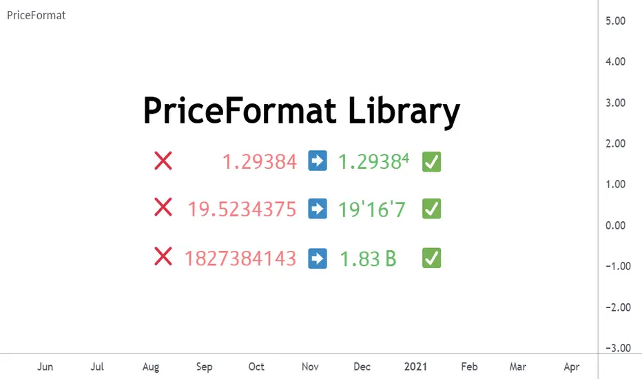
lower_tfLibrary "lower_tf"
█ OVERVIEW
This library is an enhanced (opinionated) version of the library originally developed by PineCoders contained in lower_tf .
It is a Pine Script® programming tool for advanced lower-timeframe selection and intra-bar analysis.
█ CONCEPTS
Lower Timeframe Analysis
Lower timeframe analysis refers to the analysis of price action and market microstructure using data from timeframes shorter than the current chart period. This technique allows traders and analysts to gain deeper insights into market dynamics, volume distribution, and the price movements occurring within each bar on the chart. In Pine Script®, the request.security_lower_tf() function allows this analysis by accessing intrabar data.
The library provides a comprehensive set of functions for accurate mapping of lower timeframes, dynamic precision control, and optimized historical coverage using request.security_lower_tf().
█ IMPROVEMENTS
The original library implemented ten precision levels. This enhanced version extends that to twelve levels, adding two ultra-high-precision options:
Coverage-Based Precision (Original 5 levels):
1. "Covering most chart bars (least precise)"
2. "Covering some chart bars (less precise)"
3. "Covering fewer chart bars (more precise)"
4. "Covering few chart bars (very precise)"
5. "Covering the least chart bars (most precise)"
Intrabar-Count-Based Precision (Expanded from 5 to 7 levels):
6. "~12 intrabars per chart bar"
7. "~24 intrabars per chart bar"
8. "~50 intrabars per chart bar"
9. "~100 intrabars per chart bar"
10. "~250 intrabars per chart bar"
11. "~500 intrabars per chart bar" ← NEW
12. "~1000 intrabars per chart bar" ← NEW
The key enhancements in this version include:
1. Extended Precision Range: Adds two ultra-high-precision levels (~500 and ~1000 intrabars) for advanced microstructure analysis requiring maximum granularity.
2. Market-Agnostic Implementation: Eliminates the distinction between crypto/forex and traditional markets, removing the mktFactor variable in favor of a unified, predictable approach across all asset classes.
3. Explicit Precision Mapping: Completely refactors the timeframe selection logic using native Pine Script® timeframe properties ( timeframe.isseconds , timeframe.isminutes , timeframe.isdaily , timeframe.isweekly , timeframe.ismonthly ) and explicit multiplier-based lookup tables. The original library used minute-based calculations with market-dependent conditionals that produced inconsistent results. This version provides deterministic, predictable mappings for every chart timeframe, ensuring consistent precision behavior regardless of asset type or market hours.
An example of the differences can be seen side-by-side in the chart below, where the original library is on the left and the enhanced version is on the right:
█ USAGE EXAMPLE
// This Pine Script® code is subject to the terms of the Mozilla Public License 2.0 at mozilla.org
// © andre_007
//@version=6
indicator("lower_tf Example")
import andre_007/lower_tf/1 as LTF
import PineCoders/Time/5 as PCtime
//#region ———————————————————— Example code
// ————— Constants
color WHITE = color.white
color GRAY = color.gray
string LTF1 = "Covering most chart bars (least precise)"
string LTF2 = "Covering some chart bars (less precise)"
string LTF3 = "Covering less chart bars (more precise)"
string LTF4 = "Covering few chart bars (very precise)"
string LTF5 = "Covering the least chart bars (most precise)"
string LTF6 = "~12 intrabars per chart bar"
string LTF7 = "~24 intrabars per chart bar"
string LTF8 = "~50 intrabars per chart bar"
string LTF9 = "~100 intrabars per chart bar"
string LTF10 = "~250 intrabars per chart bar"
string LTF11 = "~500 intrabars per chart bar"
string LTF12 = "~1000 intrabars per chart bar"
string TT_LTF = "This selection determines the approximate number of intrabars analyzed per chart bar. Higher numbers of
intrabars produce more granular data at the cost of less historical bar coverage, because the maximum number of
available intrabars is 200K.
\n\nThe first five options set the lower timeframe based on a specified relative level of chart bar coverage.
The last five options set the lower timeframe based on an approximate number of intrabars per chart bar."
string TAB_TXT = "Uses intrabars at the {0} timeframe.\nAvg intrabars per chart bar:
{1,number,#.#}\nChart bars covered: {2} of {3} ({4,number,#.##}%)"
string ERR_TXT = "No intrabar information exists at the {1}{0}{1} timeframe."
// ————— Inputs
string ltfModeInput = input.string(LTF3, "Intrabar precision", options = , tooltip = TT_LTF)
bool showInfoBoxInput = input.bool(true, "Show information box ")
string infoBoxSizeInput = input.string("normal", "Size ", inline = "01", options = )
string infoBoxYPosInput = input.string("bottom", "↕", inline = "01", options = )
string infoBoxXPosInput = input.string("right", "↔", inline = "01", options = )
color infoBoxColorInput = input.color(GRAY, "", inline = "01")
color infoBoxTxtColorInput = input.color(WHITE, "T", inline = "01")
// ————— Calculations
// @variable A "string" representing the lower timeframe for the data request.
// NOTE:
// This line is a good example where using `var` in the declaration can improve a script's performance.
// By using `var` here, the script calls `ltf()` only once, on the dataset's first bar, instead of redundantly
// evaluating unchanging strings on every bar. We only need one evaluation of this function because the selected
// timeframe does not change across bars in this script.
var string ltfString = LTF.ltf(ltfModeInput, LTF1, LTF2, LTF3, LTF4, LTF5, LTF6, LTF7, LTF8, LTF9, LTF10, LTF11, LTF12)
// @variable An array containing all intrabar `close` prices from the `ltfString` timeframe for the current chart bar.
array intrabarCloses = request.security_lower_tf(syminfo.tickerid, ltfString, close)
// Calculate the intrabar stats.
= LTF.ltfStats(intrabarCloses)
int chartBars = bar_index + 1
// ————— Visuals
// Plot the `avgIntrabars` and `intrabars` series in all display locations.
plot(avgIntrabars, "Average intrabars", color.silver, 6)
plot(intrabars, "Intrabars", color.blue, 2)
// Plot the `chartBarsCovered` and `chartBars` values in the Data Window and the script's status line.
plot(chartBarsCovered, "Chart bars covered", display = display.data_window + display.status_line)
plot(chartBars, "Chart bars total", display = display.data_window + display.status_line)
// Information box logic.
if showInfoBoxInput
// @variable A single-cell table that displays intrabar information.
var table infoBox = table.new(infoBoxYPosInput + "_" + infoBoxXPosInput, 1, 1)
// @variable The span of the `ltfString` timeframe formatted as a number of automatically selected time units.
string formattedLtf = PCtime.formattedNoOfPeriods(timeframe.in_seconds(ltfString) * 1000)
// @variable A "string" containing the formatted text to display in the `infoBox`.
string txt = str.format(
TAB_TXT, formattedLtf, avgIntrabars, chartBarsCovered, chartBars, chartBarsCovered / chartBars * 100, "'"
)
// Initialize the `infoBox` cell on the first bar.
if barstate.isfirst
table.cell(
infoBox, 0, 0, txt, text_color = infoBoxTxtColorInput, text_size = infoBoxSizeInput,
bgcolor = infoBoxColorInput
)
// Update the cell's text on the latest bar.
else if barstate.islast
table.cell_set_text(infoBox, 0, 0, txt)
// Raise a runtime error if no intrabar data is available.
if ta.cum(intrabars) == 0 and barstate.islast
runtime.error(str.format(ERR_TXT, ltfString, "'"))
//#endregion
█ EXPORTED FUNCTIONS
ltf(userSelection, choice1, choice2, ...)
Returns the optimal lower timeframe string based on user selection and current chart timeframe. Dynamically calculates precision to balance granularity with historical coverage within the 200K intrabar limit.
ltfStats(intrabarValues)
Analyzes an intrabar array returned by request.security_lower_tf() and returns statistics: number of intrabars in current bar, total chart bars covered, and average intrabars per bar.
█ CREDITS AND LICENSING
Original Concept : PineCoders Team
Original Lower TF Library :
License : Mozilla Public License 2.0

Qualitative and Quantitative Candlestick Score [CHE] Qualitative and Quantitative Candlestick Score
Overview
The Qualitative and Quantitative Candlestick Score is a powerful indicator for TradingView that combines both qualitative and quantitative analyses of candlestick patterns. This indicator provides traders with a comprehensive assessment of market conditions to make informed trading decisions.
Key Features
- Quantitative Analysis: Calculates a quantitative score based on the price movement of each candle.
- Qualitative Analysis: Evaluates candles based on body size, wick size, trend, and trading volume.
- Cumulative Scores: Displays cumulative green (bullish) and red (bearish) scores over a defined period.
- Trend Analysis: Identifies trend direction, strength, and provides trading recommendations (Long/Short).
- Customizable Settings: Adjust parameters for time periods, thresholds, and volume analysis.
Settings and Customizations
1. Time Period Settings:
- Period: Number of periods to calculate moving averages and cumulative scores (Default: 14).
2. Qualitative Evaluation:
- Body Size Threshold (%): Minimum size of the candle body to be considered significant (Default: 0.5%).
- Wick Size Threshold (%): Maximum size of the wicks to be considered minimal (Default: 0.3%).
3. Volume Settings:
- Include Volume in Evaluation: Whether to include trading volume in the qualitative score (Default: Enabled).
- Volume MA Period: Number of periods to calculate the moving average of volume (Default: 14).
4. Trend Settings:
- Moving Average Length: Number of periods for the Simple Moving Average used to determine the trend (Default: 50).
Calculations and Visualizations
- Quantitative Score: Difference between the closing and opening price, normalized to the opening price.
- Qualitative Score: Evaluation based on body size, wick size, trend, and volume.
- Cumulative Scores: Average of green and red scores over the defined period.
- Score Difference: Difference between cumulative green and red scores to determine trend direction.
- Trend Analysis Table: Displays trend direction, trend strength, and trading recommendation in an easy-to-read table.
Plotting and Display
- Cumulative Scores: Displays cumulative green and red scores in green and red colors.
- Score Difference: Blue line chart to visualize the difference between green and red scores.
- Zero Line: Horizontal gray line as a reference point.
- Trend Analysis Table: Table in the top right of the chart showing current trend direction, strength, and trading recommendation.
Use Cases
- Trend Identification: Use the score difference and trend analysis table to quickly assess the current market sentiment.
- Trading Recommendations: Based on the table, decide whether a long or short entry is appropriate.
- Volume Analysis: Including volume helps to better understand the strength of a trend.
Benefits
- Comprehensive Analysis: Combines quantitative and qualitative methods for a deeper market analysis.
- User-Friendly: Easy parameter adjustments allow for personalized use.
- Visually Appealing: Clear charts and tables facilitate data interpretation.
- Flexible: Adaptable to various trading strategies and timeframes.
Installation and Usage
1. Installation:
- Copy the provided Pine Script code.
- Go to TradingView and open the Pine Script Editor.
- Paste the code and save the script.
- Add the indicator to your chart.
2. Customization:
- Adjust the parameters according to your trading preferences.
- Monitor the cumulative scores and the trend analysis table for trading decisions.
Conclusion
The Qualitative and Quantitative Candlestick Score offers a comprehensive analysis of market conditions by combining quantitative and qualitative evaluation methods. With its user-friendly settings and clear visualizations, this indicator is a valuable tool for traders seeking informed and precise trading decisions.
Best regards and happy trading
Chervolino
Developed by: Chervolino
Version: 1.0
License: Free to use and customize on TradingView.
For any questions or feedback, feel free to contact me through the TradingView community.
Note: This indicator is a tool to assist with trading decisions and does not replace professional financial advice. Use it responsibly and thoroughly test it before incorporating it into your trading strategies.
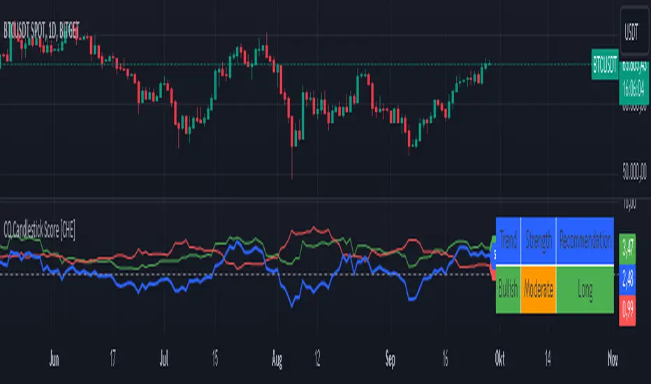
Hypothesis TF Strategy EvaluationThis script provides a statistical evaluation framework for trend-following strategies by examining whether mean returns (measured here as 1-period Rate of Change, ROC) differ significantly across different price quantile groups.
Specifically, it:
Calculates rolling 25th (Q1) and 75th (Q3) percentile levels of price over a user-defined window.
Classifies returns into three groups based on whether price is above Q3, between Q1 and Q3, or below Q1.
Computes mean returns and sample sizes for each group.
Performs Welch's t-tests (which account for unequal variances) between groups to assess if their mean returns differ significantly.
Displays results in two tables:
Summary Table: Shows mean ROC and number of observations for each group.
Hypothesis Testing Table: Shows pairwise t-statistics with significance stars for 95% and 99% confidence levels.
Key Features
Rolling quantile calculations: Captures local price distributions dynamically.
Robust hypothesis testing: Welch's t-test allows for heteroskedasticity between groups.
Significance indicators: Easy visual interpretation with "*" (95%) and "**" (99%) significance levels.
Visual aids: Plots Q1 and Q3 levels on the price chart for intuitive understanding.
Extensible and transparent: Fully commented code that emphasizes the evaluation process rather than trading signals.
Important Notes
Not a trading strategy: This script is intended as a tool for research and validation, not as a standalone trading system.
Look-ahead bias caution: The calculation carefully avoids look-ahead bias by computing quantiles and ROC values only on past data at each point.
Users must ensure look-ahead bias is removed when applying this or similar methods, as look-ahead bias would artificially inflate performance and statistical significance.
The statistical tests rely on the assumption of independent samples, which might not fully hold in financial time series but still provide useful insights
Usage Suggestions
Use this evaluation framework to validate hypotheses about the behavior of returns under different price regimes.
Integrate with your strategy development workflow to test whether certain market conditions produce statistically distinct return distributions.
Example
In this example, the script was run with a quantile length of 20 bars and a lookback of 500 bars for ROC classification.
We consider a simple hypothetical "strategy":
Go long if the previous bar closed above Q3 the 75th percentile).
Go short if the previous bar closed below Q1 (the 25th percentile).
Stay in cash if the previous close was between Q1 and Q3.
The screenshot below demonstrates the results of this evaluation. Surprisingly, the "long" group shows a negative average return, while the "short" group has a positive average return, indicating mean reversion rather than trend following.
The hypothesis testing table confirms that the only statistically significant difference (at 95% or higher confidence) is between the above Q3 and below Q1 groups, suggesting a meaningful divergence in their return behavior.
This highlights how this framework can help validate or challenge intuitive assumptions about strategy performance through rigorous statistical testing.
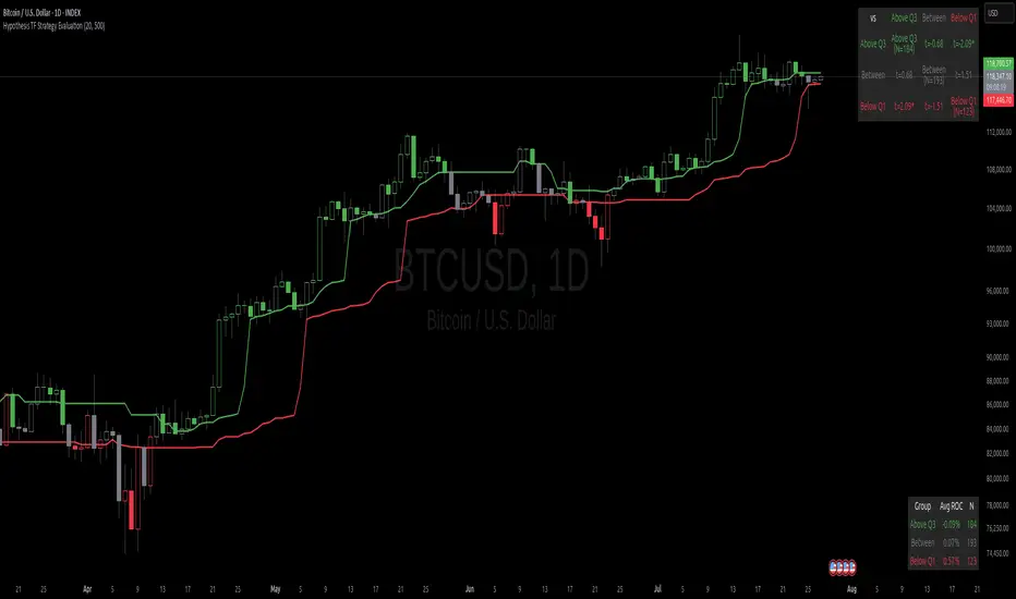
cd_sweep&cisd_CxOverview:
When the price is at a significant zone/level on a higher time frame (HTF), and it sweeps (breaks through and then closes back below/above) the high or low of the previous HTF candle, it is common to look for a Change in State of Delivery (CISD) on a lower time frame (LTF) to enter a trade.
This model can be summarized as:
HTF Sweep → LTF CISD (Optional: SMT / Divergences)
________________________________________
Working Principle & Details:
1. The indicator monitors price action on the selected HTF and tracks any sweep (violation) of the previous HTF candle's high or low. Simultaneously, it identifies CISD levels on the LTF. If SMT is enabled, it will appear as a label on the chart.
When both HTF sweep and LTF CISD conditions are met, the indicator marks the chart at the open of the next candle and triggers an alert if set.
CISD levels are tracked and updated whenever a new HTF high/low is formed.
2. The indicator monitors the formation of entry models on up to six selected pairs, displaying results in two separate tables:
o HTF Sweep Query Table: Monitors live HTF candles and reports pairs that meet the sweep condition.
o CISD Table: Displays the pairs where a valid entry model has formed. A "🔥" symbol indicates the condition has occurred.
3. Bias Visualization:
Based on the selected HTF, a visual band is shown at the bottom of the chart using the chosen bullish/bearish colors.
Bias is determined by:
o Candle closing above/below the previous one suggesting continuation.
o A failed close after a sweep implying potential reversal.
4. HTF Candles:
Displays HTF candles based on the user-defined time frame.
5. Optional SMT (Smart Money Technique):
Must be enabled in the menu and requires the correlated pair to be entered correctly for accurate results.
Displayed only as a visual confirmation, not a requirement for model formation.
If the currently open symbol sweeps the previous candle while the correlated symbol does not (or vice versa), an "SMT" label appears on the chart.
6. Color & Table Positioning:
Controlled via the settings menu.
________________________________________
Warnings:
• The indicator only marks CISDs that form at HTF high/low zones.
• Entering every time the model forms does not guarantee profitability.
• Waiting for the model to appear at significant HTF levels/zones increases the likelihood of success.
• HTF and LTF selections should follow commonly accepted combinations or user-tested time frames.
• If you want to trigger alerts only for symbols entered in the indicator, ensure the "Use indicator alerts" option is enabled.
• To set alerts for the TradingView watchlist instead, disable the "Use indicator alerts" option.
________________________________________
Feel free to share your thoughts and suggestions.
Happy trading! 💫
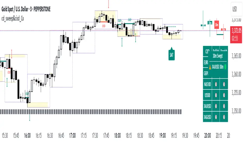
dataTableUtilitiesLibrary "dataTableUtilities"
generate_dataTable(dataTable_map, title, tableYpos, tableXpos, textSize, includes_multiple_maps, include_comments)
: Generates and shows a data table.
Parameters:
dataTable_map (map)
title (string) : (string): Title of the table
tableYpos (string) : (string): Vertical position of the table
tableXpos (string) : (string): Horizontal position of the table
textSize (string) : (string): Text size
includes_multiple_maps (bool)
include_comments (bool)
Returns: : None
generate_dataTable_multiple_columns(dataTable_map, title, tableYpos, tableXpos, textSize, includes_multiple_maps, total_columns)
: Generates and shows a data table.
Parameters:
dataTable_map (map)
title (string) : (string): Title of the table
tableYpos (string) : (string): Vertical position of the table
tableXpos (string) : (string): Horizontal position of the table
textSize (string) : (string): Text size
includes_multiple_maps (bool)
total_columns (int)
Returns: : None
BTC Dashboard D / 4H / 1H (simple)//@version=5
indicator("BTC Dashboard D / 4H / 1H (simple)", overlay = true)
// ---------- Réglages ----------
rsiLen = 14
emaLen50 = 50
emaLen200 = 200
// Petite fonction pour formater les nombres
f_fmt(float v) =>
str.tostring(v, format.mintick)
// ---------- TIMEFRAMES ----------
tfD = "D"
tf4H = "240"
tf1H = "60"
// ---------- DAILY ----------
closeD = request.security(syminfo.tickerid, tfD, close)
ema50D = request.security(syminfo.tickerid, tfD, ta.ema(close, emaLen50))
ema200D = request.security(syminfo.tickerid, tfD, ta.ema(close, emaLen200))
rsiD = request.security(syminfo.tickerid, tfD, ta.rsi(close, rsiLen))
// ---------- 4H ----------
close4H = request.security(syminfo.tickerid, tf4H, close)
ema504H = request.security(syminfo.tickerid, tf4H, ta.ema(close, emaLen50))
ema2004H = request.security(syminfo.tickerid, tf4H, ta.ema(close, emaLen200))
rsi4H = request.security(syminfo.tickerid, tf4H, ta.rsi(close, rsiLen))
// ---------- 1H ----------
close1H = request.security(syminfo.tickerid, tf1H, close)
ema501H = request.security(syminfo.tickerid, tf1H, ta.ema(close, emaLen50))
ema2001H = request.security(syminfo.tickerid, tf1H, ta.ema(close, emaLen200))
rsi1H = request.security(syminfo.tickerid, tf1H, ta.rsi(close, rsiLen))
// ---------- TABLE ----------
var table t = table.new(position.top_right, 4, 4, border_width = 1)
if barstate.islast
// Ligne d’en-tête
table.cell(t, 0, 0, "TF", text_color = color.white, bgcolor = color.new(color.black, 0))
table.cell(t, 0, 1, "Close", text_color = color.white, bgcolor = color.new(color.black, 0))
table.cell(t, 0, 2, "EMA50 / EMA200", text_color = color.white, bgcolor = color.new(color.black, 0))
table.cell(t, 0, 3, "RSI", text_color = color.white, bgcolor = color.new(color.black, 0))
// ----- DAILY -----
rowD = 1
table.cell(t, rowD, 0, "D", text_color = color.yellow, bgcolor = color.new(color.blue, 70))
table.cell(t, rowD, 1, f_fmt(closeD))
table.cell(t, rowD, 2, "50: " + f_fmt(ema50D) + "\n200: " + f_fmt(ema200D))
table.cell(t, rowD, 3, f_fmt(rsiD))
// ----- 4H -----
row4 = 2
table.cell(t, row4, 0, "4H", text_color = color.white, bgcolor = color.new(color.teal, 70))
table.cell(t, row4, 1, f_fmt(close4H))
table.cell(t, row4, 2, "50: " + f_fmt(ema504H) + "\n200: " + f_fmt(ema2004H))
table.cell(t, row4, 3, f_fmt(rsi4H))
// ----- 1H -----
row1 = 3
table.cell(t, row1, 0, "1H", text_color = color.white, bgcolor = color.new(color.green, 70))
table.cell(t, row1, 1, f_fmt(close1H))
table.cell(t, row1, 2, "50: " + f_fmt(ema501H) + "\n200: " + f_fmt(ema2001H))
table.cell(t, row1, 3, f_fmt(rsi1H))

Dee EMA 5.0
1. Indicator Features:
- The indicator can plot four different sets of EMA on a chart.
- The EMA values can be displayed on the chart with their respective names (e.g., ema9, ema20, etc.).
- The indicator allows customization of the EMA values.
2. Purpose of Dee_EMA 5.0:
- Dee_EMA 5.0 is a unique EMA indicator specially designed for traders to provide better insights and aid in trading decisions.
- The primary reason for building this indicator is to address the challenge of managing multiple time frames while using normal EMA tables.
- Traditional EMA tables might not show all EMA values across different time frames simultaneously, leading to time-consuming processes like shifting time frames and refreshing charts.
- Dee_EMA 5.0 solves this issue by displaying EMA values for different time frames in one table, allowing traders to make quick judgments without repeatedly changing time frames and refreshing charts.
3. Importance of Different Time Frame EMA Values:
- Different time frames EMA values are crucial in trading because they provide valuable insights into the market dynamics at various levels.
- When using shorter time frames (e.g., 1-minute), EMA values can help identify short-term trends, support, and resistance levels.
- On the other hand, using larger time frames (e.g., 5-minute or 15-minute) provides more data and increases the accuracy of EMA-based analysis, enabling traders to identify longer-term trends and potential price movements.
4. EMA Crossover Table:
- Traders often prefer a clutter-free chart without too many lines, but they still need access to EMA values for analysis.
- The EMA table and EMA crossover table serve this purpose by providing EMA values and EMA crossover information in a structured table format.
- With the EMA crossover table, traders can quickly check EMA values and crossovers across different time frames without having to switch time frames repeatedly, saving time and facilitating faster decision-making during trading.
In summary, Dee_EMA 5.0 is an EMA indicator designed to help traders efficiently analyze EMA values across different time frames, allowing for faster and more informed trading decisions. The EMA crossover table provides additional convenience by presenting EMA crossovers without cluttering the chart.

CNTLibraryLibrary "CNTLibrary"
Custom Functions To Help Code In Pinescript V5
Coded By Christian Nataliano
First Coded In 10/06/2023
Last Edited In 22/06/2023
Huge Shout Out To © ZenAndTheArtOfTrading and his ZenLibrary V5, Some Of The Custom Functions Were Heavily Inspired By Matt's Work & His Pine Script Mastery Course
Another Shout Out To The TradingView's Team Library ta V5
//====================================================================================================================================================
// Custom Indicator Functions
//====================================================================================================================================================
GetKAMA(KAMA_lenght, Fast_KAMA, Slow_KAMA)
Calculates An Adaptive Moving Average Based On Perry J Kaufman's Calculations
Parameters:
KAMA_lenght (int) : Is The KAMA Lenght
Fast_KAMA (int) : Is The KAMA's Fastes Moving Average
Slow_KAMA (int) : Is The KAMA's Slowest Moving Average
Returns: Float Of The KAMA's Current Calculations
GetMovingAverage(Source, Lenght, Type)
Get Custom Moving Averages Values
Parameters:
Source (float) : Of The Moving Average, Defval = close
Lenght (simple int) : Of The Moving Average, Defval = 50
Type (string) : Of The Moving Average, Defval = Exponential Moving Average
Returns: The Moving Average Calculation Based On Its Given Source, Lenght & Calculation Type (Please Call Function On Global Scope)
GetDecimals()
Calculates how many decimals are on the quote price of the current market © ZenAndTheArtOfTrading
Returns: The current decimal places on the market quote price
Truncate(number, decimalPlaces)
Truncates (cuts) excess decimal places © ZenAndTheArtOfTrading
Parameters:
number (float)
decimalPlaces (simple float)
Returns: The given number truncated to the given decimalPlaces
ToWhole(number)
Converts pips into whole numbers © ZenAndTheArtOfTrading
Parameters:
number (float)
Returns: The converted number
ToPips(number)
Converts whole numbers back into pips © ZenAndTheArtOfTrading
Parameters:
number (float)
Returns: The converted number
GetPctChange(value1, value2, lookback)
Gets the percentage change between 2 float values over a given lookback period © ZenAndTheArtOfTrading
Parameters:
value1 (float)
value2 (float)
lookback (int)
BarsAboveMA(lookback, ma)
Counts how many candles are above the MA © ZenAndTheArtOfTrading
Parameters:
lookback (int)
ma (float)
Returns: The bar count of how many recent bars are above the MA
BarsBelowMA(lookback, ma)
Counts how many candles are below the MA © ZenAndTheArtOfTrading
Parameters:
lookback (int)
ma (float)
Returns: The bar count of how many recent bars are below the EMA
BarsCrossedMA(lookback, ma)
Counts how many times the EMA was crossed recently © ZenAndTheArtOfTrading
Parameters:
lookback (int)
ma (float)
Returns: The bar count of how many times price recently crossed the EMA
GetPullbackBarCount(lookback, direction)
Counts how many green & red bars have printed recently (ie. pullback count) © ZenAndTheArtOfTrading
Parameters:
lookback (int)
direction (int)
Returns: The bar count of how many candles have retraced over the given lookback & direction
GetSwingHigh(Lookback, SwingType)
Check If Price Has Made A Recent Swing High
Parameters:
Lookback (int) : Is For The Swing High Lookback Period, Defval = 7
SwingType (int) : Is For The Swing High Type Of Identification, Defval = 1
Returns: A Bool - True If Price Has Made A Recent Swing High
GetSwingLow(Lookback, SwingType)
Check If Price Has Made A Recent Swing Low
Parameters:
Lookback (int) : Is For The Swing Low Lookback Period, Defval = 7
SwingType (int) : Is For The Swing Low Type Of Identification, Defval = 1
Returns: A Bool - True If Price Has Made A Recent Swing Low
//====================================================================================================================================================
// Custom Risk Management Functions
//====================================================================================================================================================
CalculateStopLossLevel(OrderType, Entry, StopLoss)
Calculate StopLoss Level
Parameters:
OrderType (int) : Is To Determine A Long / Short Position, Defval = 1
Entry (float) : Is The Entry Level Of The Order, Defval = na
StopLoss (float) : Is The Custom StopLoss Distance, Defval = 2x ATR Below Close
Returns: Float - The StopLoss Level In Actual Price As A
CalculateStopLossDistance(OrderType, Entry, StopLoss)
Calculate StopLoss Distance In Pips
Parameters:
OrderType (int) : Is To Determine A Long / Short Position, Defval = 1
Entry (float) : Is The Entry Level Of The Order, NEED TO INPUT PARAM
StopLoss (float) : Level Based On Previous Calculation, NEED TO INPUT PARAM
Returns: Float - The StopLoss Value In Pips
CalculateTakeProfitLevel(OrderType, Entry, StopLossDistance, RiskReward)
Calculate TakeProfit Level
Parameters:
OrderType (int) : Is To Determine A Long / Short Position, Defval = 1
Entry (float) : Is The Entry Level Of The Order, Defval = na
StopLossDistance (float)
RiskReward (float)
Returns: Float - The TakeProfit Level In Actual Price
CalculateTakeProfitDistance(OrderType, Entry, TakeProfit)
Get TakeProfit Distance In Pips
Parameters:
OrderType (int) : Is To Determine A Long / Short Position, Defval = 1
Entry (float) : Is The Entry Level Of The Order, NEED TO INPUT PARAM
TakeProfit (float) : Level Based On Previous Calculation, NEED TO INPUT PARAM
Returns: Float - The TakeProfit Value In Pips
CalculateConversionCurrency(AccountCurrency, SymbolCurrency, BaseCurrency)
Get The Conversion Currecny Between Current Account Currency & Current Pair's Quoted Currency (FOR FOREX ONLY)
Parameters:
AccountCurrency (simple string) : Is For The Account Currency Used
SymbolCurrency (simple string) : Is For The Current Symbol Currency (Front Symbol)
BaseCurrency (simple string) : Is For The Current Symbol Base Currency (Back Symbol)
Returns: Tuple Of A Bollean (Convert The Currency ?) And A String (Converted Currency)
CalculateConversionRate(ConvertCurrency, ConversionRate)
Get The Conversion Rate Between Current Account Currency & Current Pair's Quoted Currency (FOR FOREX ONLY)
Parameters:
ConvertCurrency (bool) : Is To Check If The Current Symbol Needs To Be Converted Or Not
ConversionRate (float) : Is The Quoted Price Of The Conversion Currency (Input The request.security Function Here)
Returns: Float Price Of Conversion Rate (If In The Same Currency Than Return Value Will Be 1.0)
LotSize(LotSizeSimple, Balance, Risk, SLDistance, ConversionRate)
Get Current Lot Size
Parameters:
LotSizeSimple (bool) : Is To Toggle Lot Sizing Calculation (Simple Is Good Enough For Stocks & Crypto, Whilst Complex Is For Forex)
Balance (float) : Is For The Current Account Balance To Calculate The Lot Sizing Based Off
Risk (float) : Is For The Current Risk Per Trade To Calculate The Lot Sizing Based Off
SLDistance (float) : Is The Current Position StopLoss Distance From Its Entry Price
ConversionRate (float) : Is The Currency Conversion Rate (Used For Complex Lot Sizing Only)
Returns: Float - Position Size In Units
ToLots(Units)
Converts Units To Lots
Parameters:
Units (float) : Is For How Many Units Need To Be Converted Into Lots (Minimun 1000 Units)
Returns: Float - Position Size In Lots
ToUnits(Lots)
Converts Lots To Units
Parameters:
Lots (float) : Is For How Many Lots Need To Be Converted Into Units (Minimun 0.01 Units)
Returns: Int - Position Size In Units
ToLotsInUnits(Units)
Converts Units To Lots Than Back To Units
Parameters:
Units (float) : Is For How Many Units Need To Be Converted Into Lots (Minimun 1000 Units)
Returns: Float - Position Size In Lots That Were Rounded To Units
ATRTrail(OrderType, SourceType, ATRPeriod, ATRMultiplyer, SwingLookback)
Calculate ATR Trailing Stop
Parameters:
OrderType (int) : Is To Determine A Long / Short Position, Defval = 1
SourceType (int) : Is To Determine Where To Calculate The ATR Trailing From, Defval = close
ATRPeriod (simple int) : Is To Change Its ATR Period, Defval = 20
ATRMultiplyer (float) : Is To Change Its ATR Trailing Distance, Defval = 1
SwingLookback (int) : Is To Change Its Swing HiLo Lookback (Only From Source Type 5), Defval = 7
Returns: Float - Number Of The Current ATR Trailing
DangerZone(WinRate, AvgRRR, Filter)
Calculate Danger Zone Of A Given Strategy
Parameters:
WinRate (float) : Is The Strategy WinRate
AvgRRR (float) : Is The Strategy Avg RRR
Filter (float) : Is The Minimum Profit It Needs To Be Out Of BE Zone, Defval = 3
Returns: Int - Value, 1 If Out Of Danger Zone, 0 If BE, -1 If In Danger Zone
IsQuestionableTrades(TradeTP, TradeSL)
Checks For Questionable Trades (Which Are Trades That Its TP & SL Level Got Hit At The Same Candle)
Parameters:
TradeTP (float) : Is The Trade In Question Take Profit Level
TradeSL (float) : Is The Trade In Question Stop Loss Level
Returns: Bool - True If The Last Trade Was A "Questionable Trade"
//====================================================================================================================================================
// Custom Strategy Functions
//====================================================================================================================================================
OpenLong(EntryID, LotSize, LimitPrice, StopPrice, Comment, CommentValue)
Open A Long Order Based On The Given Params
Parameters:
EntryID (string) : Is The Trade Entry ID, Defval = "Long"
LotSize (float) : Is The Lot Size Of The Trade, Defval = 1
LimitPrice (float) : Is The Limit Order Price To Set The Order At, Defval = Na / Market Order Execution
StopPrice (float) : Is The Stop Order Price To Set The Order At, Defval = Na / Market Order Execution
Comment (string) : Is The Order Comment, Defval = Long Entry Order
CommentValue (string) : Is For Custom Values In The Order Comment, Defval = Na
Returns: Void
OpenShort(EntryID, LotSize, LimitPrice, StopPrice, Comment, CommentValue)
Open A Short Order Based On The Given Params
Parameters:
EntryID (string) : Is The Trade Entry ID, Defval = "Short"
LotSize (float) : Is The Lot Size Of The Trade, Defval = 1
LimitPrice (float) : Is The Limit Order Price To Set The Order At, Defval = Na / Market Order Execution
StopPrice (float) : Is The Stop Order Price To Set The Order At, Defval = Na / Market Order Execution
Comment (string) : Is The Order Comment, Defval = Short Entry Order
CommentValue (string) : Is For Custom Values In The Order Comment, Defval = Na
Returns: Void
TP_SLExit(FromID, TPLevel, SLLevel, PercentageClose, Comment, CommentValue)
Exits Based On Predetermined TP & SL Levels
Parameters:
FromID (string) : Is The Trade ID That The TP & SL Levels Be Palced
TPLevel (float) : Is The Take Profit Level
SLLevel (float) : Is The StopLoss Level
PercentageClose (float) : Is The Amount To Close The Order At (In Percentage) Defval = 100
Comment (string) : Is The Order Comment, Defval = Exit Order
CommentValue (string) : Is For Custom Values In The Order Comment, Defval = Na
Returns: Void
CloseLong(ExitID, PercentageClose, Comment, CommentValue, Instant)
Exits A Long Order Based On A Specified Condition
Parameters:
ExitID (string) : Is The Trade ID That Will Be Closed, Defval = "Long"
PercentageClose (float) : Is The Amount To Close The Order At (In Percentage) Defval = 100
Comment (string) : Is The Order Comment, Defval = Exit Order
CommentValue (string) : Is For Custom Values In The Order Comment, Defval = Na
Instant (bool) : Is For Exit Execution Type, Defval = false
Returns: Void
CloseShort(ExitID, PercentageClose, Comment, CommentValue, Instant)
Exits A Short Order Based On A Specified Condition
Parameters:
ExitID (string) : Is The Trade ID That Will Be Closed, Defval = "Short"
PercentageClose (float) : Is The Amount To Close The Order At (In Percentage) Defval = 100
Comment (string) : Is The Order Comment, Defval = Exit Order
CommentValue (string) : Is For Custom Values In The Order Comment, Defval = Na
Instant (bool) : Is For Exit Execution Type, Defval = false
Returns: Void
BrokerCheck(Broker)
Checks Traded Broker With Current Loaded Chart Broker
Parameters:
Broker (string) : Is The Current Broker That Is Traded
Returns: Bool - True If Current Traded Broker Is Same As Loaded Chart Broker
OpenPC(LicenseID, OrderType, UseLimit, LimitPrice, SymbolPrefix, Symbol, SymbolSuffix, Risk, SL, TP, OrderComment, Spread)
Compiles Given Parameters Into An Alert String Format To Open Trades Using Pine Connector
Parameters:
LicenseID (string) : Is The Users PineConnector LicenseID
OrderType (int) : Is The Desired OrderType To Open
UseLimit (bool) : Is If We Want To Enter The Position At Exactly The Previous Closing Price
LimitPrice (float) : Is The Limit Price Of The Trade (Only For Pending Orders)
SymbolPrefix (string) : Is The Current Symbol Prefix (If Any)
Symbol (string) : Is The Traded Symbol
SymbolSuffix (string) : Is The Current Symbol Suffix (If Any)
Risk (float) : Is The Trade Risk Per Trade / Fixed Lot Sizing
SL (float) : Is The Trade SL In Price / In Pips
TP (float) : Is The Trade TP In Price / In Pips
OrderComment (string) : Is The Executed Trade Comment
Spread (float) : is The Maximum Spread For Execution
Returns: String - Pine Connector Order Syntax Alert Message
ClosePC(LicenseID, OrderType, SymbolPrefix, Symbol, SymbolSuffix)
Compiles Given Parameters Into An Alert String Format To Close Trades Using Pine Connector
Parameters:
LicenseID (string) : Is The Users PineConnector LicenseID
OrderType (int) : Is The Desired OrderType To Close
SymbolPrefix (string) : Is The Current Symbol Prefix (If Any)
Symbol (string) : Is The Traded Symbol
SymbolSuffix (string) : Is The Current Symbol Suffix (If Any)
Returns: String - Pine Connector Order Syntax Alert Message
//====================================================================================================================================================
// Custom Backtesting Calculation Functions
//====================================================================================================================================================
CalculatePNL(EntryPrice, ExitPrice, LotSize, ConversionRate)
Calculates Trade PNL Based On Entry, Eixt & Lot Size
Parameters:
EntryPrice (float) : Is The Trade Entry
ExitPrice (float) : Is The Trade Exit
LotSize (float) : Is The Trade Sizing
ConversionRate (float) : Is The Currency Conversion Rate (Used For Complex Lot Sizing Only)
Returns: Float - The Current Trade PNL
UpdateBalance(PrevBalance, PNL)
Updates The Previous Ginve Balance To The Next PNL
Parameters:
PrevBalance (float) : Is The Previous Balance To Be Updated
PNL (float) : Is The Current Trade PNL To Be Added
Returns: Float - The Current Updated PNL
CalculateSlpComm(PNL, MaxRate)
Calculates Random Slippage & Commisions Fees Based On The Parameters
Parameters:
PNL (float) : Is The Current Trade PNL
MaxRate (float) : Is The Upper Limit (In Percentage) Of The Randomized Fee
Returns: Float - A Percentage Fee Of The Current Trade PNL
UpdateDD(MaxBalance, Balance)
Calculates & Updates The DD Based On Its Given Parameters
Parameters:
MaxBalance (float) : Is The Maximum Balance Ever Recorded
Balance (float) : Is The Current Account Balance
Returns: Float - The Current Strategy DD
CalculateWR(TotalTrades, LongID, ShortID)
Calculate The Total, Long & Short Trades Win Rate
Parameters:
TotalTrades (int) : Are The Current Total Trades That The Strategy Has Taken
LongID (string) : Is The Order ID Of The Long Trades Of The Strategy
ShortID (string) : Is The Order ID Of The Short Trades Of The Strategy
Returns: Tuple Of Long WR%, Short WR%, Total WR%, Total Winning Trades, Total Losing Trades, Total Long Trades & Total Short Trades
CalculateAvgRRR(WinTrades, LossTrades)
Calculates The Overall Strategy Avg Risk Reward Ratio
Parameters:
WinTrades (int) : Are The Strategy Winning Trades
LossTrades (int) : Are The Strategy Losing Trades
Returns: Float - The Average RRR Values
CAGR(StartTime, StartPrice, EndTime, EndPrice)
Calculates The CAGR Over The Given Time Period © TradingView
Parameters:
StartTime (int) : Is The Starting Time Of The Calculation
StartPrice (float) : Is The Starting Price Of The Calculation
EndTime (int) : Is The Ending Time Of The Calculation
EndPrice (float) : Is The Ending Price Of The Calculation
Returns: Float - The CAGR Values
//====================================================================================================================================================
// Custom Plot Functions
//====================================================================================================================================================
EditLabels(LabelID, X1, Y1, Text, Color, TextColor, EditCondition, DeleteCondition)
Edit / Delete Labels
Parameters:
LabelID (label) : Is The ID Of The Selected Label
X1 (int) : Is The X1 Coordinate IN BARINDEX Xloc
Y1 (float) : Is The Y1 Coordinate IN PRICE Yloc
Text (string) : Is The Text Than Wants To Be Written In The Label
Color (color) : Is The Color Value Change Of The Label Text
TextColor (color)
EditCondition (int) : Is The Edit Condition of The Line (Setting Location / Color)
DeleteCondition (bool) : Is The Delete Condition Of The Line If Ture Deletes The Prev Itteration Of The Line
Returns: Void
EditLine(LineID, X1, Y1, X2, Y2, Color, EditCondition, DeleteCondition)
Edit / Delete Lines
Parameters:
LineID (line) : Is The ID Of The Selected Line
X1 (int) : Is The X1 Coordinate IN BARINDEX Xloc
Y1 (float) : Is The Y1 Coordinate IN PRICE Yloc
X2 (int) : Is The X2 Coordinate IN BARINDEX Xloc
Y2 (float) : Is The Y2 Coordinate IN PRICE Yloc
Color (color) : Is The Color Value Change Of The Line
EditCondition (int) : Is The Edit Condition of The Line (Setting Location / Color)
DeleteCondition (bool) : Is The Delete Condition Of The Line If Ture Deletes The Prev Itteration Of The Line
Returns: Void
//====================================================================================================================================================
// Custom Display Functions (Using Tables)
//====================================================================================================================================================
FillTable(TableID, Column, Row, Title, Value, BgColor, TextColor, ToolTip)
Filling The Selected Table With The Inputed Information
Parameters:
TableID (table) : Is The Table ID That Wants To Be Edited
Column (int) : Is The Current Column Of The Table That Wants To Be Edited
Row (int) : Is The Current Row Of The Table That Wants To Be Edited
Title (string) : Is The String Title Of The Current Cell Table
Value (string) : Is The String Value Of The Current Cell Table
BgColor (color) : Is The Selected Color For The Current Table
TextColor (color) : Is The Selected Color For The Current Table
ToolTip (string) : Is The ToolTip Of The Current Cell In The Table
Returns: Void
DisplayBTResults(TableID, BgColor, TextColor, StartingBalance, Balance, DollarReturn, TotalPips, MaxDD)
Filling The Selected Table With The Inputed Information
Parameters:
TableID (table) : Is The Table ID That Wants To Be Edited
BgColor (color) : Is The Selected Color For The Current Table
TextColor (color) : Is The Selected Color For The Current Table
StartingBalance (float) : Is The Account Starting Balance
Balance (float)
DollarReturn (float) : Is The Account Dollar Reture
TotalPips (float) : Is The Total Pips Gained / loss
MaxDD (float) : Is The Maximum Drawdown Over The Backtesting Period
Returns: Void
DisplayBTResultsV2(TableID, BgColor, TextColor, TotalWR, QTCount, LongWR, ShortWR, InitialCapital, CumProfit, CumFee, AvgRRR, MaxDD, CAGR, MeanDD)
Filling The Selected Table With The Inputed Information
Parameters:
TableID (table) : Is The Table ID That Wants To Be Edited
BgColor (color) : Is The Selected Color For The Current Table
TextColor (color) : Is The Selected Color For The Current Table
TotalWR (float) : Is The Strategy Total WR In %
QTCount (int) : Is The Strategy Questionable Trades Count
LongWR (float) : Is The Strategy Total WR In %
ShortWR (float) : Is The Strategy Total WR In %
InitialCapital (float) : Is The Strategy Initial Starting Capital
CumProfit (float) : Is The Strategy Ending Cumulative Profit
CumFee (float) : Is The Strategy Ending Cumulative Fee (Based On Randomized Fee Assumptions)
AvgRRR (float) : Is The Strategy Average Risk Reward Ratio
MaxDD (float) : Is The Strategy Maximum DrawDown In Its Backtesting Period
CAGR (float) : Is The Strategy Compounded Average GRowth In %
MeanDD (float) : Is The Strategy Mean / Average Drawdown In The Backtesting Period
Returns: Void
//====================================================================================================================================================
// Custom Pattern Detection Functions
//====================================================================================================================================================
BullFib(priceLow, priceHigh, fibRatio)
Calculates A Bullish Fibonacci Value (From Swing Low To High) © ZenAndTheArtOfTrading
Parameters:
priceLow (float)
priceHigh (float)
fibRatio (float)
Returns: The Fibonacci Value Of The Given Ratio Between The Two Price Points
BearFib(priceLow, priceHigh, fibRatio)
Calculates A Bearish Fibonacci Value (From Swing High To Low) © ZenAndTheArtOfTrading
Parameters:
priceLow (float)
priceHigh (float)
fibRatio (float)
Returns: The Fibonacci Value Of The Given Ratio Between The Two Price Points
GetBodySize()
Gets The Current Candle Body Size IN POINTS © ZenAndTheArtOfTrading
Returns: The Current Candle Body Size IN POINTS
GetTopWickSize()
Gets The Current Candle Top Wick Size IN POINTS © ZenAndTheArtOfTrading
Returns: The Current Candle Top Wick Size IN POINTS
GetBottomWickSize()
Gets The Current Candle Bottom Wick Size IN POINTS © ZenAndTheArtOfTrading
Returns: The Current Candle Bottom Wick Size IN POINTS
GetBodyPercent()
Gets The Current Candle Body Size As A Percentage Of Its Entire Size Including Its Wicks © ZenAndTheArtOfTrading
Returns: The Current Candle Body Size IN PERCENTAGE
GetTopWickPercent()
Gets The Current Top Wick Size As A Percentage Of Its Entire Body Size
Returns: Float - The Current Candle Top Wick Size IN PERCENTAGE
GetBottomWickPercent()
Gets The Current Bottom Wick Size As A Percentage Of Its Entire Bodu Size
Returns: Float - The Current Candle Bottom Size IN PERCENTAGE
BullishEC(Allowance, RejectionWickSize, EngulfWick, NearSwings, SwingLookBack)
Checks If The Current Bar Is A Bullish Engulfing Candle
Parameters:
Allowance (int) : To Give Flexibility Of Engulfing Pattern Detection In Markets That Have Micro Gaps, Defval = 0
RejectionWickSize (float) : To Filter Out long (Upper And Lower) Wick From The Bullsih Engulfing Pattern, Defval = na
EngulfWick (bool) : To Specify If We Want The Pattern To Also Engulf Its Upper & Lower Previous Wicks, Defval = false
NearSwings (bool) : To Specify If We Want The Pattern To Be Near A Recent Swing Low, Defval = true
SwingLookBack (int) : To Specify How Many Bars Back To Detect A Recent Swing Low, Defval = 10
Returns: Bool - True If The Current Bar Matches The Requirements of a Bullish Engulfing Candle
BearishEC(Allowance, RejectionWickSize, EngulfWick, NearSwings, SwingLookBack)
Checks If The Current Bar Is A Bearish Engulfing Candle
Parameters:
Allowance (int) : To Give Flexibility Of Engulfing Pattern Detection In Markets That Have Micro Gaps, Defval = 0
RejectionWickSize (float) : To Filter Out long (Upper And Lower) Wick From The Bearish Engulfing Pattern, Defval = na
EngulfWick (bool) : To Specify If We Want The Pattern To Also Engulf Its Upper & Lower Previous Wicks, Defval = false
NearSwings (bool) : To Specify If We Want The Pattern To Be Near A Recent Swing High, Defval = true
SwingLookBack (int) : To Specify How Many Bars Back To Detect A Recent Swing High, Defval = 10
Returns: Bool - True If The Current Bar Matches The Requirements of a Bearish Engulfing Candle
Hammer(Fib, ColorMatch, NearSwings, SwingLookBack, ATRFilterCheck, ATRPeriod)
Checks If The Current Bar Is A Hammer Candle
Parameters:
Fib (float) : To Specify Which Fibonacci Ratio To Use When Determining The Hammer Candle, Defval = 0.382 Ratio
ColorMatch (bool) : To Filter Only Bullish Closed Hammer Candle Pattern, Defval = false
NearSwings (bool) : To Specify If We Want The Doji To Be Near A Recent Swing Low, Defval = true
SwingLookBack (int) : To Specify How Many Bars Back To Detect A Recent Swing Low, Defval = 10
ATRFilterCheck (float) : To Filter Smaller Hammer Candles That Might Be Better Classified As A Doji Candle, Defval = 1
ATRPeriod (simple int) : To Change ATR Period Of The ATR Filter, Defval = 20
Returns: Bool - True If The Current Bar Matches The Requirements of a Hammer Candle
Star(Fib, ColorMatch, NearSwings, SwingLookBack, ATRFilterCheck, ATRPeriod)
Checks If The Current Bar Is A Hammer Candle
Parameters:
Fib (float) : To Specify Which Fibonacci Ratio To Use When Determining The Hammer Candle, Defval = 0.382 Ratio
ColorMatch (bool) : To Filter Only Bullish Closed Hammer Candle Pattern, Defval = false
NearSwings (bool) : To Specify If We Want The Doji To Be Near A Recent Swing Low, Defval = true
SwingLookBack (int) : To Specify How Many Bars Back To Detect A Recent Swing Low, Defval = 10
ATRFilterCheck (float) : To Filter Smaller Hammer Candles That Might Be Better Classified As A Doji Candle, Defval = 1
ATRPeriod (simple int) : To Change ATR Period Of The ATR Filter, Defval = 20
Returns: Bool - True If The Current Bar Matches The Requirements of a Hammer Candle
Doji(MaxWickSize, MaxBodySize, DojiType, NearSwings, SwingLookBack)
Checks If The Current Bar Is A Doji Candle
Parameters:
MaxWickSize (float) : To Specify The Maximum Lenght Of Its Upper & Lower Wick, Defval = 2
MaxBodySize (float) : To Specify The Maximum Lenght Of Its Candle Body IN PERCENT, Defval = 0.05
DojiType (int)
NearSwings (bool) : To Specify If We Want The Doji To Be Near A Recent Swing High / Low (Only In Dragonlyf / Gravestone Mode), Defval = true
SwingLookBack (int) : To Specify How Many Bars Back To Detect A Recent Swing High / Low (Only In Dragonlyf / Gravestone Mode), Defval = 10
Returns: Bool - True If The Current Bar Matches The Requirements of a Doji Candle
BullishIB(Allowance, RejectionWickSize, EngulfWick, NearSwings, SwingLookBack)
Checks If The Current Bar Is A Bullish Harami Candle
Parameters:
Allowance (int) : To Give Flexibility Of Harami Pattern Detection In Markets That Have Micro Gaps, Defval = 0
RejectionWickSize (float) : To Filter Out long (Upper And Lower) Wick From The Bullsih Harami Pattern, Defval = na
EngulfWick (bool) : To Specify If We Want The Pattern To Also Engulf Its Upper & Lower Previous Wicks, Defval = false
NearSwings (bool) : To Specify If We Want The Pattern To Be Near A Recent Swing Low, Defval = true
SwingLookBack (int) : To Specify How Many Bars Back To Detect A Recent Swing Low, Defval = 10
Returns: Bool - True If The Current Bar Matches The Requirements of a Bullish Harami Candle
BearishIB(Allowance, RejectionWickSize, EngulfWick, NearSwings, SwingLookBack)
Checks If The Current Bar Is A Bullish Harami Candle
Parameters:
Allowance (int) : To Give Flexibility Of Harami Pattern Detection In Markets That Have Micro Gaps, Defval = 0
RejectionWickSize (float) : To Filter Out long (Upper And Lower) Wick From The Bearish Harami Pattern, Defval = na
EngulfWick (bool) : To Specify If We Want The Pattern To Also Engulf Its Upper & Lower Previous Wicks, Defval = false
NearSwings (bool) : To Specify If We Want The Pattern To Be Near A Recent Swing High, Defval = true
SwingLookBack (int) : To Specify How Many Bars Back To Detect A Recent Swing High, Defval = 10
Returns: Bool - True If The Current Bar Matches The Requirements of a Bearish Harami Candle
//====================================================================================================================================================
// Custom Time Functions
//====================================================================================================================================================
BarInSession(sess, useFilter)
Determines if the current price bar falls inside the specified session © ZenAndTheArtOfTrading
Parameters:
sess (simple string)
useFilter (bool)
Returns: A boolean - true if the current bar falls within the given time session
BarOutSession(sess, useFilter)
Determines if the current price bar falls outside the specified session © ZenAndTheArtOfTrading
Parameters:
sess (simple string)
useFilter (bool)
Returns: A boolean - true if the current bar falls outside the given time session
DateFilter(startTime, endTime)
Determines if this bar's time falls within date filter range © ZenAndTheArtOfTrading
Parameters:
startTime (int)
endTime (int)
Returns: A boolean - true if the current bar falls within the given dates
DayFilter(monday, tuesday, wednesday, thursday, friday, saturday, sunday)
Checks if the current bar's day is in the list of given days to analyze © ZenAndTheArtOfTrading
Parameters:
monday (bool)
tuesday (bool)
wednesday (bool)
thursday (bool)
friday (bool)
saturday (bool)
sunday (bool)
Returns: A boolean - true if the current bar's day is one of the given days
AUSSess()
Checks If The Current Australian Forex Session In Running
Returns: Bool - True If Currently The Australian Session Is Running
ASIASess()
Checks If The Current Asian Forex Session In Running
Returns: Bool - True If Currently The Asian Session Is Running
EURSess()
Checks If The Current European Forex Session In Running
Returns: Bool - True If Currently The European Session Is Running
USSess()
Checks If The Current US Forex Session In Running
Returns: Bool - True If Currently The US Session Is Running
UNIXToDate(Time, ConversionType, TimeZone)
Converts UNIX Time To Datetime
Parameters:
Time (int) : Is The UNIX Time Input
ConversionType (int) : Is The Datetime Output Format, Defval = DD-MM-YYYY
TimeZone (string) : Is To Convert The Outputed Datetime Into The Specified Time Zone, Defval = Exchange Time Zone
Returns: String - String Of Datetime

Streamer WatermarkThis unique indicator doesn’t help you trade but it makes your charts look super clean and professional in images and live streams! This indicator works by displaying two tables. The first table has day of the week, date, and free form text. The second table has ticker symbol and timeframe of the current chart.
Everything about the tables and the cells is completely controllable by the user! Here is a breakdown of how customizable the user can make this indicator:
Table:
Toggle each table to be displayed on or off
Move each table into 9 different locations around the chart
Move each table separately
Table background color and transparency
Table border color and transparency
Table border width
Table frame width
Cells:
Each cell can be individually toggled on or off (the table will resize dynamically)
Cell text color and transparency
Text size with 6 different options
Date format with 12 different formats
Input Text:
Text
Emoji
Text & emojis
ASCII characters
Symbols
Anything that can by copied and pasted
Any combination of the above
Notes
Use text size “Auto” if viewing the same chart on desktop and on smart phone (Auto makes the text scale based upon screen size)
Gallery
Disclaimer
Please read the TradingView House Rules carefully before using this indicator to add text, symbols, characters, or anything else to your charts and posting on TradingView Ideas or Scripts. This indicator and the author are not responsible for users not reading, fully understanding, and abiding by TradingView’s House Rules. Please watermark responsibly.

DebugLibrary "Debug"
Some debugging functions.
label_on_each_bar(txt, y_position, label_size, label_color, txt_color)
Prints a label on every bar to show text. By default, only the last 50 labels will be shown on the chart. You can increase this amount up to a maximum of 500 by using the max_labels_count parameter in your script’s indicator() or strategy() declaration statement.
Parameters:
txt (string) : New label text.
y_position (float) : New price of the label position.
label_size (string) : Possible values: size.auto, size.tiny, size.small, size.normal, size.large, size.huge. Optional. Default value is `size.small`.
label_color (color) : New label border and arrow color. Optional. Default value is `color.blue`.
txt_color (color) : New text color. Optional. Default value is `color.white`.
Returns: void
label_on_last_bar(txt, y_position, label_size, label_color, txt_color, txt_align)
Prints one label at last bar to show text.
Parameters:
txt (string) : New label text.
y_position (float) : New price of the label position.
label_size (string) : Possible values: size.auto, size.tiny, size.small, size.normal, size.large, size.huge. Optional. Default value is `size.large`.
label_color (color) : New label border and arrow color. Optional. Default value is `color.blue`.
txt_color (color) : New text color. Optional. Default value is `color.white`.
txt_align (string) : Label text alignment. Optional. Possible values: text.align_left, text.align_center, text.align_right. Default value is `text.align_center`.
Returns: void
table_symbol_informations(table_position, table_color, text_color)
Prints a table to show all the Symbol information, including its function names.
Parameters:
table_position (string) : Position of the table. Optional. Possible values are: position.top_left, position.top_center, position.top_right, position.middle_left, position.middle_center, position.middle_right, position.bottom_left, position.bottom_center, position.bottom_right. Default value is `position.middle_right`.
table_color (color) : The background color of the table. Optional. The default is `color.yellow`.
text_color (color) : The color of the text. Optional. The default is `color.black`.
Returns: void
table_array_float(array_float, table_columns, table_rows, table_position, table_color, txt_color, txt_size)
Prints a table to show float values of an array.
Parameters:
array_float (float ) : The array that will be showed.
table_columns (int)
table_rows (int) : The number of rows to show the values.
table_position (string) : Position of the table. Optional. Possible values are: position.top_left, position.top_center, position.top_right, position.middle_left, position.middle_center, position.middle_right, position.bottom_left, position.bottom_center, position.bottom_right. Default value is `position.bottom_center`.
table_color (color) : The background color of the table. Optional. By default there is no color.
txt_color (color)
txt_size (string) : Possible values: size.auto, size.tiny, size.small, size.normal, size.large, size.huge. Optional. Default value is `size.normal`.
Returns: void
table_array_int(array_float, table_columns, table_rows, table_position, table_color, txt_color, txt_size)
Prints a table to show int values of an array.
Parameters:
array_float (int ) : The array that will be showed.
table_columns (int)
table_rows (int) : The number of rows to show the values.
table_position (string) : Position of the table. Optional. Possible values are: position.top_left, position.top_center, position.top_right, position.middle_left, position.middle_center, position.middle_right, position.bottom_left, position.bottom_center, position.bottom_right. Default value is `position.bottom_center`.
table_color (color) : The background color of the table. Optional. By default there is no color.
txt_color (color)
txt_size (string) : Possible values: size.auto, size.tiny, size.small, size.normal, size.large, size.huge. Optional. Default value is `size.normal`.
Returns: void
